Optical absorption for interband and intersubband transitions

Section author: Takuma Sato

Input Files:

• QWIP_singleQW_GaAs_AlGaAs_nnp.in

• QWIP_singleQW_InAs_AlSb_nnp.in

• QWIP_Gunapala_JAP_1991_nnp.in

• AlGaAs_QW_Frankenberger_Simple_nnp.in

• AlGaAs_QW_Frankenberger_Simple_nnp_fast.in

• AlGaAs_QW_Frankenberger_Doping_schottky07_nnp.in

• AlGaAs_QW_Frankenberger_Doping_schottky07_nnp_fast.in

Contents

In this tutorial we illustrate the optics{ } module to demonstrate what nextnano++ can simulate for optoelectronic devices. This module performs a detailed calculation to optical absorption phenomena, using 8 (or 6) band $\mathbf{k}\cdot \mathbf{p}$ models. If you are interested in

• the background physics of this module and how to write the input file, go to Principle and nextnano++ implementation.

• the simulation results for intersubband transitions, go to 1D tutorial for intersubband transitions: Quantum well infrared photodetector.

• the simulation results for interband transitions, go to 1D tutorial for interband transitions: Frankenberger.

• optical absorption in 2D devices, (under construction)

• optical absorption in broken-gap structures, (under construction)

This algorithm is implemented based on the following diploma thesis:

• Thomas Eißfeller, Linear Optical Response of Semiconductor Nanodevices, Technische Universität München (2008)

For the physics of optical transition in semiconductors and its application, we refer to

• Shun L. Chuang, Physics of Optoelectronic Devices (Wiley, 1995)

• S.M. Sze & Kwok K. Ng, Physics of Semiconductor Devices (Wiley, 2007)

Principle and nextnano++ implementation

${\mathbf{k}}_{\parallel }$ space

In the k.p analysis of one- (or two-) dimensional structures we have a projection of the Bloch wave vector along translation-invariant directions. We denote them as ${\mathbf{k}}_{\parallel }=k_y\hat{y}+k_z\hat{z}$ (1D) and ${\mathbf{k}}_{\parallel }=k_z\hat{z}$ (2D). Under envelope function approximation the $\mathbf{k}\cdot \mathbf{p}$ model yields the following equation to determine the confined states in structured directions

(2.4.49)$$\sum _{\mu =1}^8{H}_{\nu \mu }^{\mathrm{kp}8}({\mathbf{k}}_{\parallel },{\mathbf{r}}_{\perp })f_{m,\mu }({\mathbf{r}}_{\perp })=E_m({\mathbf{k}}_{\parallel })f_{m,\nu }({\mathbf{r}}_{\perp })(\nu =1,\dots ,8),$$

where the Greek indices label the k.p bands and $m$ denotes eigenvalues, ${\mathbf{r}}_{\perp }=x\hat{x}$ in 1D and ${\mathbf{r}}_{\perp }=x\hat{x}+y\hat{y}$ in 2D. $H^{\mathrm{kp}8}$ is the 8 $\times$ 8 matrix whose elements are given by the k.p parameters in the database. $f_{m,\mu }({\mathbf{r}}_{\perp })‘$ are the envelopes in the structured directions. The full wave function is given at each ${\mathbf{k}}_{\parallel }$ as

(2.4.50)$${\mathrm{\Psi }}_n({\mathbf{k}}_{\parallel },\mathbf{r})=\sum _{\mu =1}^8{F}_{m,\mu }({\mathbf{k}}_{\parallel },\mathbf{r})u_{\mu }(\mathbf{r})=\sum _{\mu =1}^8\frac{e^{i{\mathbf{k}}_{\parallel }\cdot {\mathbf{r}}_{\parallel }}}{\sqrt{A}}{f}_{m,\mu }({\mathbf{r}}_{\perp })u_{\mu }(\mathbf{r}),$$

where $u_{\mu }(\mathbf{r})$ is the Bloch function of the band $\mu$ at $\mathbf{k}=0$ and $A=\int d{\mathbf{r}}_{\parallel }$. In general, both the conduction band ($\mathrm{\Gamma }$) and valence bands contribute to this full wave function. The spinor composition is exported to Quantum\spinor_composition. After solving this “Schrödinger” equation, the wave function is integrated over a limited region in ${\mathbf{k}}_{\parallel }$ space to obtain the charge density, which is used in the quantum-current-Poisson iteration. The region is specified under quantum{ } as

quantum{
  region{
      kp_8band{
        k_integration{
            relative_size = $r_quantum     # size of k||-space in quantum{ } (relative to the Brillouin zone)
            num_points    = $N_quantum     # number of k|| points where Schrödinger eq. is solved
            num_subpoints = $Nsub_quantum  # number of points between k|| points where wave functions and eigenvalues are interpolated
            force_k0_subspace =            # (optional) use the eigenfunctions of the Schrödinger equation at k=0 as the basis for the Schrödinger equation at all k-point (default: no)
        }
      }
  }
}

Note

When force_k0_subspace=yes in quantum{ } or optics{ }, the Schrödinger equations at non-zero k-points are solved in the subspace of the eigenfunctions obtained by the Schrödinger equation at ${\mathbf{k}}_{\parallel }=0$. This approximation largely improves the computational speed. In case you are planning to use this approximation for final results, please make sure to check whether the resulting loss of accuracy in density is acceptable (quantum{ }) or the loss in optical spectra is acceptable (optics{ }).

Optical absorption spectrum

When 1) Schrödinger equation is solved with k.p method, 2) optics{ } flag is present and 3) the specifier optics{ } is present under run{ } flag, nextnano++ calculates the absorption spectrum.

optics{
  region{
  ...          # see below for details
  }
}

run{
  quantum{ }
  optics{ }
}

The optical absorption accompanied by excitation of charge carriers (state $n\to m$) in a condensed matter is calculated from Fermi’s golden rule [ChuangOpto1995]. The absorption coefficient has the dimension of (length)${}^{-1}$.

(2.4.51)$$\alpha (\overrightarrow{ϵ},\omega )=\frac{\pi e^2}{n_{s}c{\epsilon }_0{m}_0^2\omega }\frac{1}{V}\sum _{n>m}\sum _{{\mathbf{k}}_{\parallel }}|\overrightarrow{ϵ}\cdot {\overrightarrow{\pi }}_{nm}({\mathbf{k}}_{\parallel }){|}^2(f_m-f_n)\delta (E_n-E_m-\hslash \omega ),$$

where the first sum runs over bands that fulfill $E_n>E_m$, and $f_m({\mathbf{k}}_{\parallel })=[1+e^{[E_m({\mathbf{k}}_{\parallel })-E_F]/k_{B}T}{]}^{-1}$ is the occupation of eigenstate $m$. When optics{ occupation_ignore=yes } (default is no), the program assumes

$$\begin{array}{r}\{\begin{array}{l}{f}_m({\mathbf{k}}_{\parallel })=0\text{if}m\in \text{conduction band}\\ f_m({\mathbf{k}}_{\parallel })=1\text{if}m\in \text{valence band}\end{array}\end{array}$$

The light polarization $\overrightarrow{ϵ}$ and refractive index $n_s$ are specified in the input file. The refractive index is in general frequency-dependent, but we assume it to be constant and equal to the substrate value.

optics{
  region{
      polarization{ name="TM" re = [1,0,0] }    # in 1D simulation, x is the growth direction
      polarization{ name="TE" re = [0,1,0] }    # complex (circular) polarization is also allowed

      refractive_index =               # (optional) use alternative value for the refractive index (default: substrate value)
  }
}

The core of the optical transition is the optical matrix elements $\overrightarrow{ϵ}\cdot {\overrightarrow{\pi }}_{nm}({\mathbf{k}}_{\parallel })$ because the kinematic momentum operator $\overrightarrow{\pi }=({\pi }_x,{\pi }_y,{\pi }_z)$ couples linearly to the vector potential that accounts for the electromagnetic field. Here $\overrightarrow{\pi }$ is the sum of the conventional momentum operator $\mathbf{p}$ and the contribution of spin-orbit interaction. The optical matrix elements are calculated as

(2.4.52)$$\begin{array}{r}{\overrightarrow{\pi }}_{nm}({\mathbf{k}}_{\parallel })=⟨n|\overrightarrow{\pi }|m⟩=\int d\mathbf{r}\left(\begin{array}{ccc}{F}_{n1}^{\ast }& \cdots & F_{n8}^{\ast }\end{array}\right)\left(\begin{array}{ccc}& & \\ & {\overrightarrow{\pi }}_{\nu \mu }^{\mathrm{kp}8}& \\ & & \end{array}\right)\left(\begin{array}{c}{F}_{m1}\\ ⋮\\ F_{m8}\end{array}\right),\end{array}$$

where the 8$\times$8 matrix representation of the momentum operator, ${\overrightarrow{\pi }}_{\nu \mu }^{\mathrm{kp}8}$, has been derived using the Hellmann-Feynman theorem extended to the 8-band k.p model up to first order in $\mathbf{k}$ [Eißfeller]. For the analysis of the absorption spectrum, nextnano++ also prints out some fractions of the absorption coefficient formula in the output folder, namely

1. occupation (if output_occupations=yes) \Optics\occupation_~.dat $f_m({\mathbf{k}}_{\parallel })$

2. eigenvalue dispersion (if output_energies=yes) \Optics\energy_disp_~.dat $E_m({\mathbf{k}}_{\parallel })$

3. transition intensity (if output_transitions=yes) Optics\transition_disp_~.dat $T_{nm}(\overrightarrow{ϵ},{\mathbf{k}}_{\parallel })=\frac{2}{m_0}|\overrightarrow{ϵ}\cdot {\overrightarrow{\pi }}_{nm}({\mathbf{k}}_{\parallel }){|}^2$

4. imaginary part of the dielectric function for each transition (if output_spectra{ output_components yes }) \Optics\imepsilon_~.dat $\mathrm{Im}{\epsilon }_{nm}(\overrightarrow{ϵ},\omega )=\frac{m_0}{2{\omega }^2}\frac{\pi e^2}{m_0^2{\epsilon }_0}\frac{1}{V}\sum _{{\mathbf{k}}_{\parallel }}{T}_{nm}(\overrightarrow{ϵ},{\mathbf{k}}_{\parallel })(f_m-f_n)\delta (E_n-E_m-\hslash \omega )$

5. total imaginary part of the dielectric function \Optics\imepsilon_~.dat $\mathrm{Im}\epsilon (\overrightarrow{ϵ},\omega )=\sum _{n>m}\mathrm{Im}{\epsilon }_{nm}(\overrightarrow{ϵ},\omega )$

6. total absorption spectrum \Optics\absorption_~.dat $\alpha (\overrightarrow{ϵ},\omega )=\sum _{n>m}{\alpha }_{nm}(\overrightarrow{ϵ},\omega )=\sum _{n>m}\frac{\omega }{n_{s}c}\mathrm{Im}{\epsilon }_{nm}(\overrightarrow{ϵ},\omega )$

The following part of the input specifies how much transitions to be taken into account. The setting for k_integration{} is explained in the next section.

optics{
  region{
      interband = $INTERBAND    # yes or no
      intraband = $INTRABAND    # yes or no

      energy_min        = $ENERGY_MIN          # minimum energy of the absorption spectrum
      energy_max        = $ENERGY_MAX          # maximum energy of the absorption spectrum
      energy_resolution = $ENERGY_RESOLUTION   # energy grid spacing

      k_integration{
        relative_size = $r_optics     # size of k||-space in optics{ } (relative to the Brillouin zone)
        num_points    = $N_optics     # number of k|| points where transition intensities are computed
        num_subpoints = $Nsub_optics  # number of points between k|| points where transition intensity is interpolated
        force_k0_subspace =           # (optional) use the eigenfunctions of the Schrödinger equation at k=0 as the basis for the Schrödinger equation at all k-point (default: no)
      }
  }
}

Parameters in k_integration{} (for fine tuning)

Parameters in k_integration{} in optics{ } flag (hereafter $r_{\mathrm{opt}},N_{\mathrm{opt}},N_{\mathrm{opt}}^{\prime }$) specify the size and resolution of the ${\mathbf{k}}_{\parallel }$ space integration in absorption spectrum calculation, $\sum _{{\mathbf{k}}_{\parallel }}$. This should not be confused with the specifier k_integration{} in quantum{ } flag used for quantum mechanical charge density integration (hereafter $r_q,N_q,N_q^{\prime }$, see Figure 2.4.305).

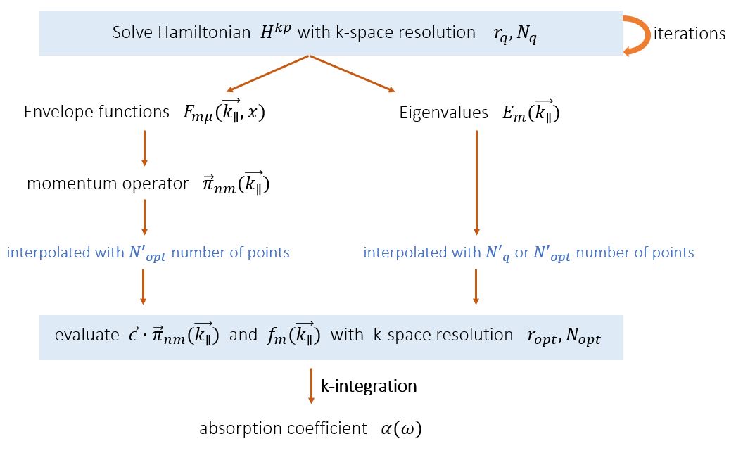
Figure 2.4.305 Calculation algorithm of optical absorption spectrum and its relation to the parameters in k_integration{}. $r_q,N_q,N_q^{\prime }$ and $r_{\mathrm{opt}},N_{\mathrm{opt}},N_{\mathrm{opt}}^{\prime }$ are specified in quantum{ } and optics{ }, respectively. To do; the energy dispersion is interpolated with $N_{\mathrm{q}}^{\prime }$ or $N_{\mathrm{opt}}^{\prime }$?

First we discuss the parameters $r_{\mathrm{opt}}$ and $N_{\mathrm{opt}}$. The size of k|| space may affect the validity of simulation results. It also determines the simulation load. Here are some hints to determine the appropriate parameter sets:

• In undoped systems, integrating up to $|{\mathbf{k}}_{\parallel }|$ that gives in-plane kinetic energy ${\hslash }^2{k}_{\parallel }^2/2m$ corresponding to $2k_{B}T$ or $3k_{B}T$ should be sufficient. Usually $r_{\mathrm{opt}}=0.3$ is sufficiently large to include all occupied states. In doped systems, it depends on the Fermi energy.

• To see the range of occupied states in ${\mathbf{k}}_{\parallel }$ space, run a simulation and look at the output \Optics\occupation_~.dat. We recommend checking the box “Show grid” on the left panel in Output tab of nextnanomat (see also Output). This shows the occupation $f_m({\mathbf{k}}_{\parallel })$ as a function of ${\mathbf{k}}_{\parallel }$. Let us consider 1D simulation and suppose you got the following:

where $(r_{\mathrm{opt}},N_{\mathrm{opt}})=(0.3,8)$. The horizontal- and vertical axes are $k_y$ and $k_z$, respectively. The area $|k_{y,z}|\le r_{\mathrm{opt}}\frac{\pi }{a}$ is shown with the k||-space gridding (thin white lines). The number of k|| points in one direction is $2N_{\mathrm{opt}}+3$. The occupation profile is not smooth, and you might want a higher resolution by increasing the parameter $(r_{\mathrm{opt}},N_{\mathrm{opt}})\to (0.3,60)$:

The occupation becomes smooth, but at the same time this significantly increases the number of k points (in 1D simulation, (the number of k points)$\propto (r_{\mathrm{opt}}{N}_{\mathrm{opt}}{)}^2$). Noting that the black region, where occupation is zero, does not contribute to the absorption, you can “zoom in” to the colored region by decreasing $r_{\mathrm{opt}}$ and $N_{\mathrm{opt}}$ in such a way that the ratio $r_{\mathrm{opt}}/N_{\mathrm{opt}}$ remains constant. This will cut down the irrelevant region without changing the resolution. For example, if you set $(r_{\mathrm{opt}},N_{\mathrm{opt}})=(0.05,10)$, you obtain

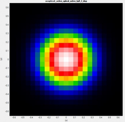
and this should be sufficient for the k||-space integration.

After tuning the parameters $r_{\mathrm{opt}},N_{\mathrm{opt}}$, we can further optimize the setting regarding the interpolation. The number of subpoints $N_{\mathrm{opt}}^{\prime }$ determines at how many k|| points the transition intensity should be interpolated. Increasing $N_{\mathrm{opt}}^{\prime }$ gives $E_m({\mathbf{k}}_{\parallel })$ of higher resolution and makes the absorption spectrum smooth. Figure 2.4.306 shows that this parameter improves the absorption spectrum.

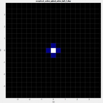
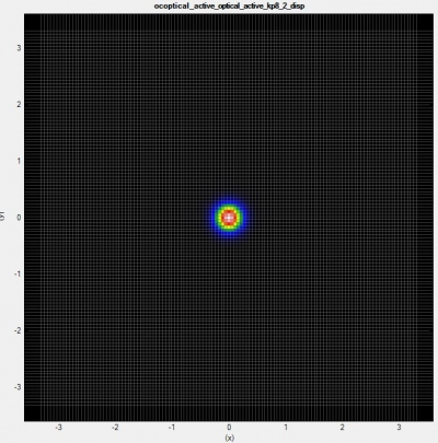
Figure 2.4.306 The effect of the parameter $N_{\mathrm{opt}}^{\prime }$ specified in optics{ k_integration{}} on absorption spectrum output \Optics\absorption. Larger $N_{\mathrm{opt}}^{\prime }$ smoothens the k||-dependence of the integrand, which leads to smoother spectrum.

To do: investigate spin_degeneracy=yes/no and dipole_approximation = yes/no

1D tutorial for intersubband transitions: Quantum well infrared photodetector

In the following we apply the formalism to several devices. As a first example, we model the absorption spectrum of an AlGaAs/GaAs quantum well infrared photodetector (QWIP). The QWIP is based on photoconductivity due to intersubband excitation.

Input files

• QWIP_singleQW_GaAs_AlGaAs_nnp.in

• QWIP_singleQW_InAs_AlSb_nnp.in

• QWIP_Gunapala_JAP_1991_nnp.in

The first example uses the same parameters used in

• FIG. 20 in B.F. Levine, J. Appl. Phys. 74 (8), 15 (1993),

while the third example is based on [GunapalaJAP1991]

GaAs/AlGaAs single QW - band structure, eigenstates and absorption

We first illustrate the first example QWIP_singleQW_GaAs_AlGaAs_nnp.in. In this example, we model optical absorption in single quantum well structure. The following input is required for self-consistent quantum-current-Poisson simulation:

quantum{
  region{
      name = "optical_active"
      no_density = no
      kp_8band{
        num_electrons = $OptNumE
        num_holes     = $OptNumH
      }
  }
}

poisson{ }

current{}

run{
  strain{ }            # strain calculation
  current_poisson{ }
  quantum_current_poisson{ }
  optics{ }            # absorption calculation
}

The specifier no_density=no lets the program calculate quantum mechanical charge density (default). Current-Poisson equation takes over this value. The band structure and wave functions are shown in Figure 2.4.307 and Figure 2.4.308, respectively.

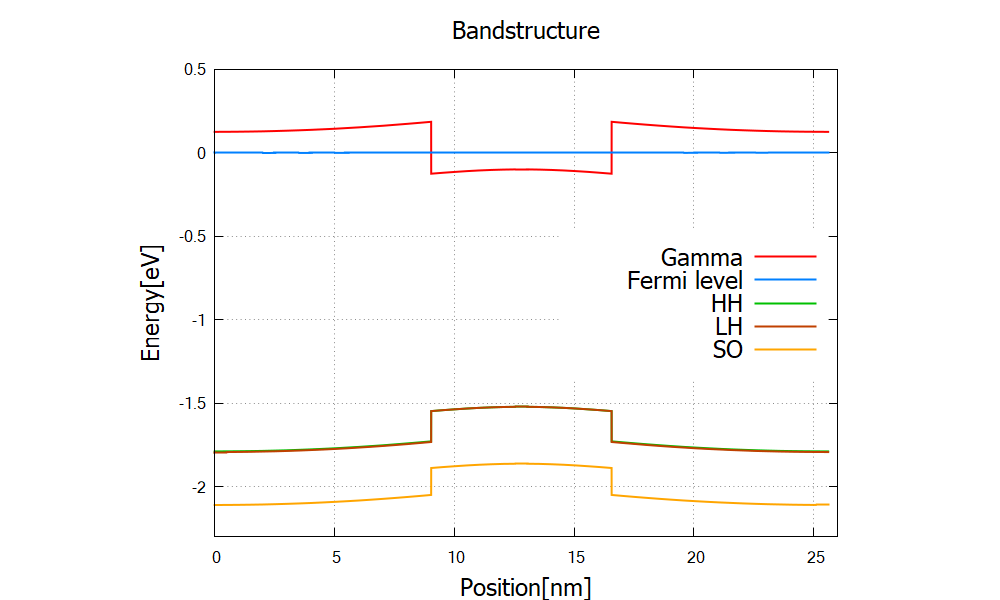
Figure 2.4.307 Single quantum well structure \bandedges.dat. The bias voltage between two contacts is set to 2mV.

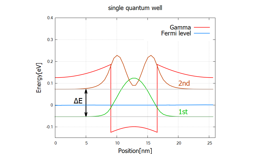
Figure 2.4.308 Probability distribution $|\psi (x){|}^2$ of the confined states at ${\mathbf{k}}_{\parallel }=0$ (\Quantum\probabilities_shift_optical_active). The wave functions here are the solution to the 8-band k.p model. The energy separation is $\mathrm{\Delta }E$=0.06960-(-0.05589)=0.1255[eV] according to the output data. The electron Fermi energy lies between two bound states.

The output folder \Optics contains computed absorption spectra. Let us first check the occupation $f_m({\mathbf{k}}_{\parallel })$ used in the calculation. When comparing the results \Optics\occupation, please mind the autoscale mode of nextnanomat:

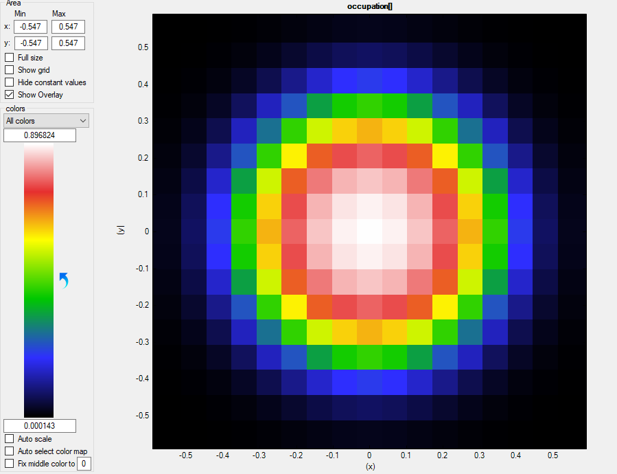
Figure 2.4.309 Occupation of the first (m=1) bound states as a function of ${\mathbf{k}}_{\parallel }$.

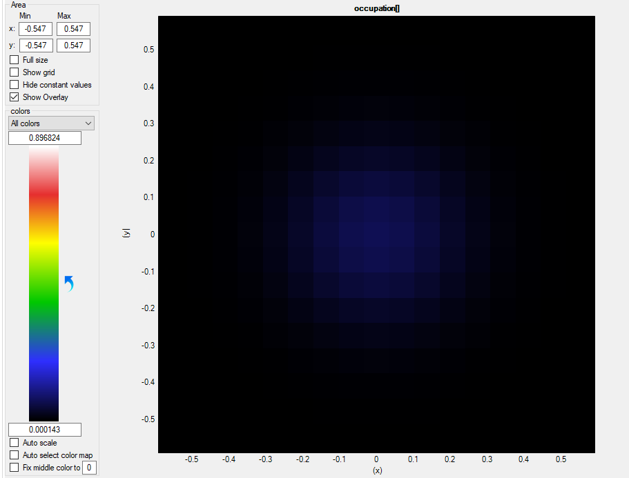
Figure 2.4.310 Occupation of the second (m=2) bound states as a function of ${\mathbf{k}}_{\parallel }$.

The autoscale mode in nextnanomat is set off here. We clearly see that the first state is well occupied, whereas for the second state is not (precisely speaking $f_1(0)$=0.897 while $f_2(0)$<0.07).

The absorption coefficient for TE ($\overrightarrow{ϵ}=\hat{y}$) and TM ($\overrightarrow{ϵ}=\hat{x}$) light polarization is shown in Figure 2.4.311. The energy grid spacing here is $ENERGY_RESOLUTION=0.5meV. For single-band models the peak becomes very sharp unless one introduces phenomenological broadening function such as Lorentzian. In k.p calculation, in contrast, peaks gets broadened because the transition energies, $E_n({\mathbf{k}}_{\parallel })-E_m({\mathbf{k}}_{\parallel })$, depends on k||. One can confirm this by comparing the output \Optics\energy_disp_~.dat for states m=1 and 2 (not shown). In intersubband transitions the transition energies can be concave downward in k|| space, i.e., $E_n({\mathbf{k}}_{\parallel })-E_m({\mathbf{k}}_{\parallel })\propto -k^2$, depending on the masses. In the present case the absorption spectrum has a tail in the region $\hslash \omega <\mathrm{\Delta }E$.

Figure 2.4.311 Absorption coefficient in \Optics\absorption_~.dat as a function of photon energy, for TE and TM. Black arrow points the energy separation $\mathrm{\Delta }E$. The broadening of the spectrum is due to the k||-dependence of wave functions and corresponding eigenvalues.

The optical transitions between conduction band states (intersubband transitions) in response to TE-polarized light is only allowed when eigenstates have finite spinor components in valence bands. In the present case its large band gap and small confinement leads to small band-mixing, rendering TE absorption spectrum orders of magnitude smaller than TM polarization (Figure 2.4.311). As seen in the output \Quantum\spinor_composition_~.dat, eigenstates contain approximately 98% contribution from conduction band and 2% from valence band.

InAs/AlSb single QW - small band gap & large confinement

In the second example QWIP_singleQW_InAs_AlSb_nnp.in, single quantum well is narrower and the band gap is smaller than the first example. The small band gap and large confinement of the wave function (Figure 2.4.312) leads to large band mixing. In fact, the output \Quantum\spinor_composition_~.dat shows that the ground states in Figure Figure 2.4.312 consists of 80.7% of conduction band and 19.3% of valence band contribution.

Figure 2.4.312 Confined states at ${\mathbf{k}}_{\parallel }=0$ (\Quantum\probabilities_shift_optical_active) in a narrower and deeper quantum well. The blue line marks the electron Fermi energy (0eV).

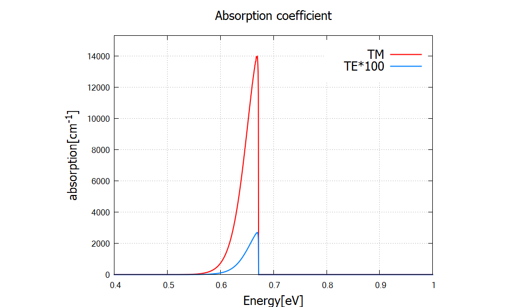
Figure 2.4.313 Absorption spectrum for TE and TM. TE absorption becomes relevant compared to Figure 2.4.311 because of the large band-mixing. Note that TE spectrum here is multiplied by a factor of 100, instead of 1000 in Figure 2.4.311.

Periodic case

In the third example QWIP_Gunapala_JAP_1991_nnp.in, we set the bias to zero and impose the periodic boundary condition. The GaAs/Al${}_x$Ga${}_{1-x}$As superlattice structure induces miniband states below the barriers, enabling bound-to-continuum absorptions of sub-eV photons. This $\mu \mathrm{m}$-wavelength photodetector works without electron tunneling through the barriers, thereby improving the detectivity [Gunapala]. The band structure bandedges.dat and wave functions \Quantum\probabilities_shift.dat are shown in Figure 2.4.314. We have continuum states above the barriers as well as bound states in the superlattice (miniband).

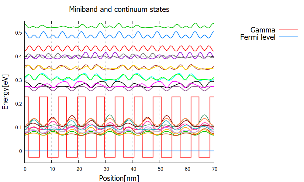
Figure 2.4.314 Gamma band profile and probability distribution of the bound miniband states and continuum states above the top of the barriers.

The absorption coefficient is exported to \Optics\absorption. The indices in the filename *_kp8_TE_m_n.dat refer to the transition from state m to state n. The files without indices contain the total absorption spectrum (sum over all transitions). The total absorption spectrum for TE and TM polarization looks like this:

Figure 2.4.315 Absorption spectrum for TE ($\overrightarrow{ϵ}=\hat{y}$) and TM ($\overrightarrow{ϵ}=\hat{x}$) polarization. TE spectrum is magnified by factor of 1000. We observe that TM absorption is much larger than TE, while the peak positions are the same.

The peak positions do not depend on polarization, while the peak height is much larger for TM polarization compared to the one for TE. Looking at the absorption spectrum for each transition, we identify which transition contributes to which peak (Figure 2.4.316).

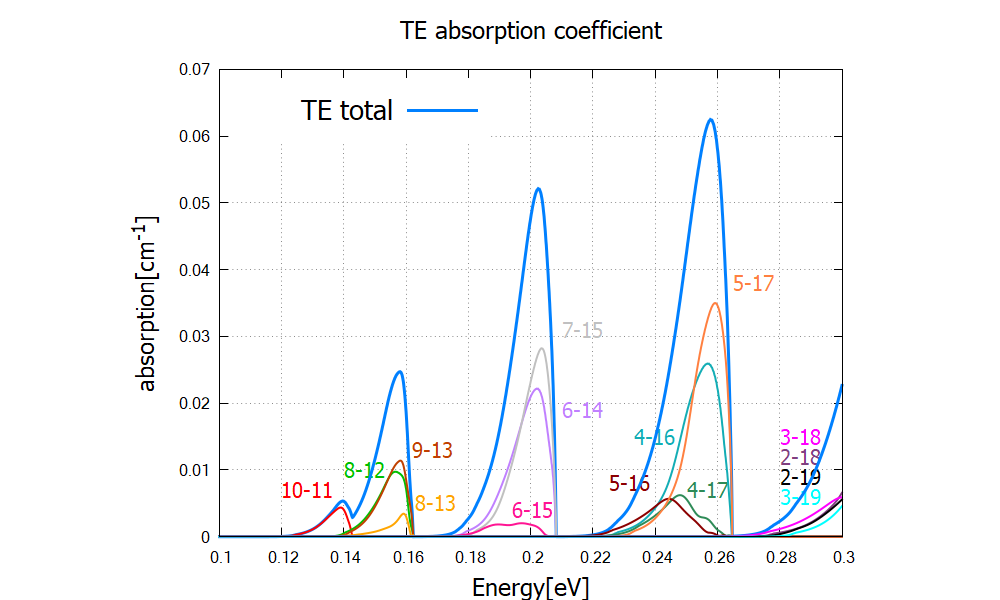
Figure 2.4.316 Contributions from different transitions to the total TE absorption spectrum.

Let us look at the eigenvalue and occupation of each state to confirm this result. The eigenvalues of the bound- and continuum states are written in the output \Quantum\probabilities_shift.dat or \Quantum\energy_spectrum.

Note

quantum{ } uses spin-resolved index for the eigenstates, so there are 80 states in total. In optics{ }, however, two spin-degenerate states are summed up and there are only 40 states. This number (1 to 40) is used in the \Optics output filenames. For the consistency, we use the latter notation throughout. (To do: examine the specifier spin_degeneracy)

Based on the indices in Figure 2.4.316, we identify the first four peaks to the following four different transitions (Figure 2.4.317). We have confirmed that the peak energies in Figure 2.4.316 are consistent to the energy separation of the corresponding states.

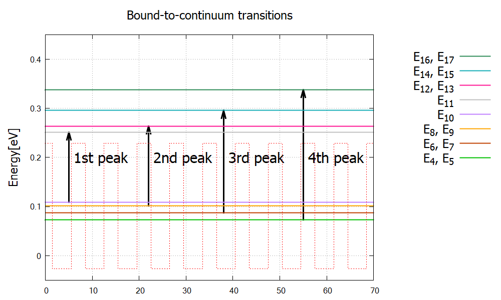
Figure 2.4.317 Eigenenergies of relevant bound- and continuum states. Many other transitions have little contribution due to the shape of the wave functions and/or occupation of the states. When we calculate for wider energy range, i.e. increase the parameter $ENERGY_MAX, there will be many more peaks that are attributed to higher energy transitions.

Lastly we check the occupation (Fermi-Dirac distribution) $f_m({\mathbf{k}}_{\parallel })$. In the output \Optics\eigenvaluespectrum (Figure 2.4.318), occupation at k||=0 of $m$-th state, $f_m({\mathbf{k}}_{\parallel }=0)$, is plotted at corresponding eigenvalues $E_m$. The function takes the maximum value at the origin ${\mathbf{k}}_{\parallel }=0$. In the present system, $f_1(0)=0.087,f_2(0)=0.077,\dots ,f_{10}(0)=0.0148$ for the bound states, whereas $f_m(0)<{10}^{-4}$ for continuum states ($m\ge 11$). Therefore the initial states in Figure 2.4.317 are well occupied and the final states are mostly empty. This enables optical absorption via bound-to-continuum excitation of electrons, thereby realizing a quantum well photodetector with high detectivity.

Figure 2.4.318 Occupation of eigenstates showing a noticeable difference for bound (m=1-10) and continuum (m=11,…) states.

1D tutorial for interband transitions: Frankenberger

Input files

• AlGaAs_QW_Frankenberger_Simple_nnp.in

• AlGaAs_QW_Frankenberger_Simple_nnp_fast.in

• AlGaAs_QW_Frankenberger_Doping_schottky07_nnp.in

• AlGaAs_QW_Frankenberger_Doping_schottky07_nnp_fast.in

These files are located in the sample files folder. The fast examples reduce the computation load by limiting exact solution only to $k=0$ point and computing all other $k$ points in the basis of the $k=0$ wave functions (force_k0_subspace; see quantum{ } and optics{ } documentations).

Optical absorption and interband transitions

In the input file AlGaAs_QW_Frankenberger_Simple_nnp.in, we consider a single quantum well structure:

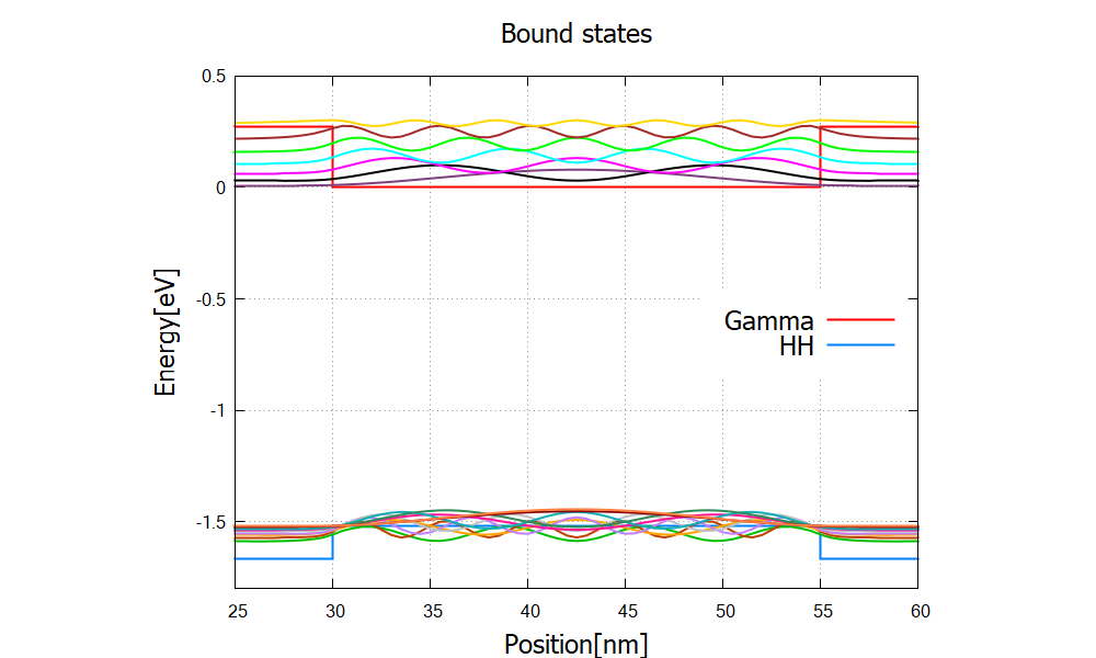
Figure 2.4.319 The conduction band edge profile (bandedges.dat) and wave functions of the bound states (\Quantum\probabilities_shift).

The program solves the 8-band k.p model coupled to the Poisson equation to find the eigenstates and compute the absorption coefficient. Figure Figure 2.4.320 shows the absorption spectrum for circularly polarized light ($\overrightarrow{ϵ}=\hat{y}-i\hat{z}$). In contrast to QWIP examples above, peaks have long tails toward higher energy. This is because the transition energies $E_n({\mathbf{k}}_{\parallel })-E_m({\mathbf{k}}_{\parallel })$ in interband transitions are concave upward $\sim +k^2$ (here we do not consider Type 2 semiconductors).

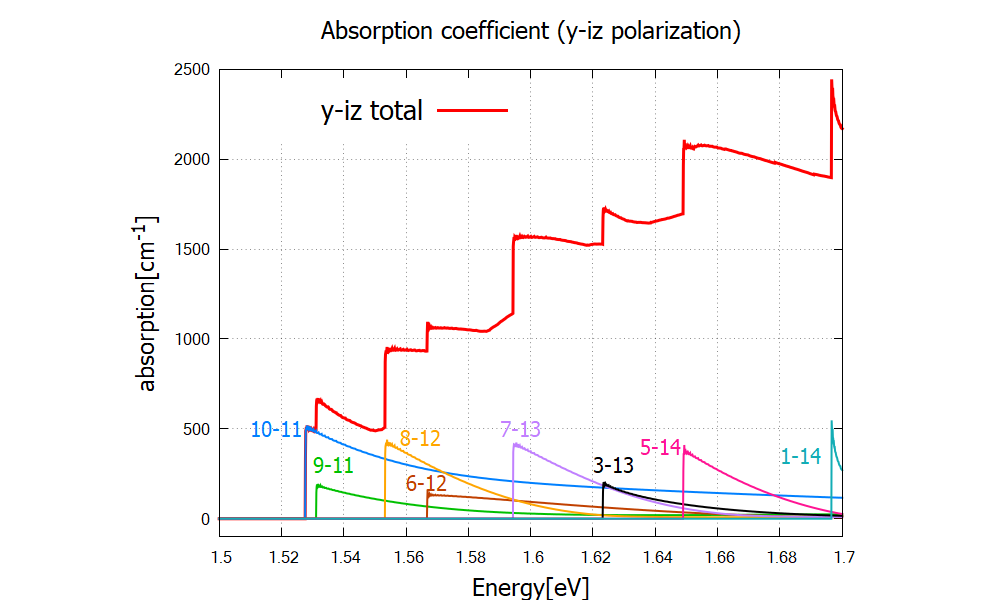
Figure 2.4.320 Absorption coefficient of circularly polarized lights. Numbers “m-n” denote each transition $m\to n$. The first four transitions are sketched in Figure 2.4.321 .

The steps of this absorption spectrum are associated with the following interband transitions:

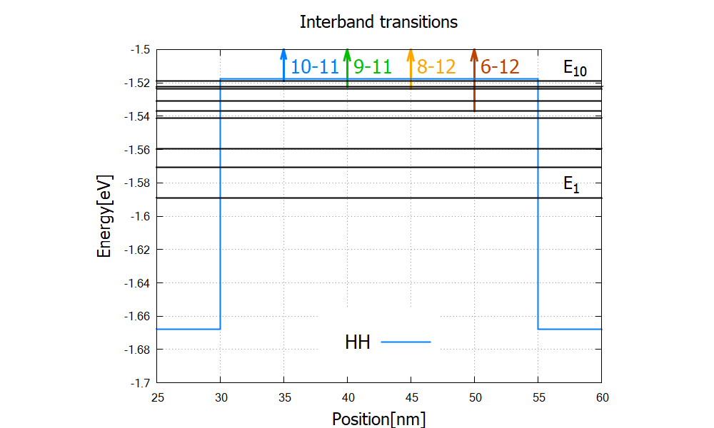
Figure 2.4.321 Eigenvalues (black) and transitions from valence-band to conduction band bound states (arrows) which are responsible for the first four steps in Figure 2.4.320. Here spin-degenerate states are counted as one state (eigenstate numbering in optics{ }).

Note

In the end of the log file, you find the message “Integration reliable up to —eV”. This tells you up to which energy the absorption spectrum is reliable. Since we only consider the vicinity of the origin ${\mathbf{k}}_{\parallel }=0$, the reliable energy interval is bound from above by the energy difference of the initial and final states at the edge of the k||-space considered. The upper limit d [eV] is given by

$d=\underset{{\mathbf{k}}_{\parallel }\in {\mathrm{\Omega }}^{\ast }\mathrm{edge}}{min}|E_n({\mathbf{k}}_{\parallel })-E_m({\mathbf{k}}_{\parallel })|$

where ${\mathrm{\Omega }}^{\ast }$ is the region in k||-space specified in optics{ region{ k_integration{} } } with parameters $r_{\mathrm{opt}}$ and $N_{\mathrm{opt}}$. In the present case d=3.2eV, while the calculation is safely performed for the interval [1.4, 1.7] (eV). This message appears only when interband transitions are computed, i.e. when interband=yes and intraband=no in optics{ } flag.

Doping and Schottkey barrier

In the second input file AlGaAs_QW_Frankenberger_Doping_schottky07_nnp.in, we consider the following structure:

Figure 2.4.322 The band structure and eigen functions used for optics calculation. The Fermi level is at 0eV.

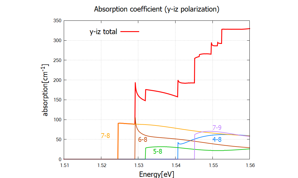
Figure 2.4.323 Absorption coefficient of circularly polarized lights. Numbers “m-n” denote each transition $m\to n$.

Figure 2.4.324 compares the results for different settings for occupation $f_m({\mathbf{k}}_{\parallel })$. When optics{ occupation_ignore=yes }, valence bands and conduction bands are considered to be fully occupied and fully empty, respectively. When the actual occupation of eigenstates are taken into account, in contrast, optical transitions to conduction band states just above the Fermi energy are prohibited because of the thermal distribution of electrons.

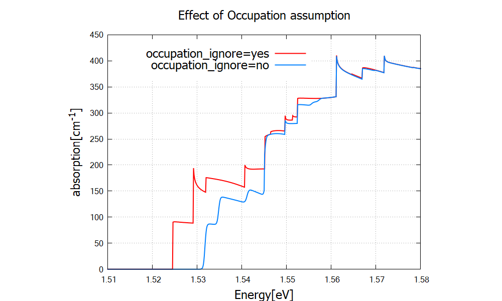
Figure 2.4.324 Absorption coefficient for different settings of occupation. The red curve is identical to the total absorption spectrum in Figure 2.4.323. When occupation_ignore=no, absorption of low energy photons is suppressed due to the occupation of the lowest conduction band states (also see Figure 2.4.322).

---

Last update: nn/nn/nnnn