Hole wave functions in a quantum wire subjected to a magnetic field
Attention
This tutorial is under construction
- Input files:
QWR-magnetic-field_InAs_2D_sg_nnp.in
QWR-magnetic-field_InAs_2D_6kp_nnp.in
- Scope:
This tutorial aims to calculate the hole wavefunctions in a quantum wire, which is subject to an applied magnetic field.
- Output files:
bias_00000/Quantum/energy_spectrum_quantum_region_HH_00000.dat
bias_00000/Quantum/probabilities_quantum_region_HH.fld
bias_00000/Quantum/energy_spectrum_quantum_region_kp6_00000.dat
bias_00000/Quantum/probabilities_quantum_region_kp6_00000.fld
Structure
Similar to the 1D confinement in a quantum well, it is possible to confine electrons or holes in two dimensions, i.e. in a quantum wire. The quantum wire structure which is simulated in this tutorial is depicted in Figure 2.4.544. The quantum wire consists of InAs (blue area) and is confined by GaAs barriers (red area). Its size is 10 nm x 10 nm whereas the whole simulation dimension is 30 nm x 30 nm.
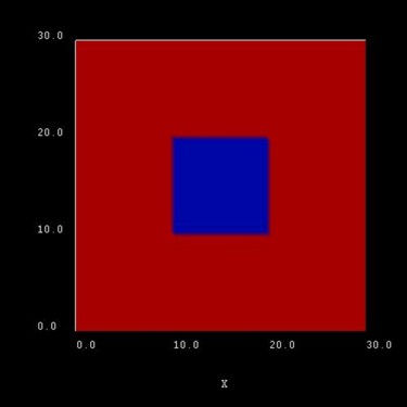
Figure 2.4.544 Simulated quantum wire (blue region) consisting of InAs surrounded by GaAs (red).
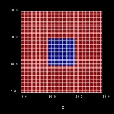
Figure 2.4.545 Possible configuration of rectangular grid lines. Here, the grid spacing is 0.5 nm, thus the quantum wire (blue area) consists of 21 x 21 = 400 grid points.
In our simulations we apply Dirichlet boundary conditions to the quantum region (
The energy levels and the wave functions of a rectangular quantum wire of length 10 nm with infinite barriers can be calculated analytically. This way we can compare our numerical calculations to analytical results. A discussion of the analytical solution of the 2D Schrödinger equation of a particle in a rectangle (i.e. quantum wire) with infinite barriers can be found in e.g. [MitinKochelapStroscio1999].
The potential inside the quantum wire is assumed to be 0 eV. As effective mass we take the isotropic heavy hole effective mass of InAs, i.e.
where
where
Generally, the energy levels are not degenerate, i.e. all energies are different. However, some energy levels with different quantum numbers coincide, if the lengths along two directions are identical (
The calculated eigenvalues for the 10 nm quadratic quantum wire can be found in the file bias_00000/Quantum/energy_spectrum_quantum_region_HH_00000.dat. The numerical results obtained by nextnano++ with 0.10 nm grid spacing are:
The differences between the analytical and numerical results are highlighted in red.
Single-band effective-mass approximation
The corresponding input file is QWR-magnetic-field_InAs_2D_sg_nnp.in
Hole wave functions (without magnetic field)
To turn off the magnetic field in the simulation, the variable $magnetic_field_on should be set to 0 in the input file.
The following figures show the probability densities
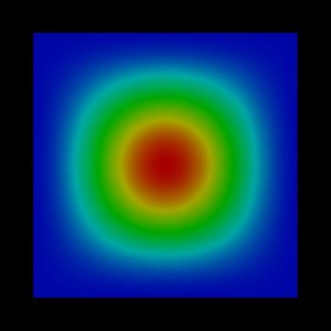
Figure 2.4.546 Probability density
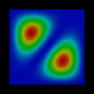
Figure 2.4.547 Probability density

Figure 2.4.548 Probability density
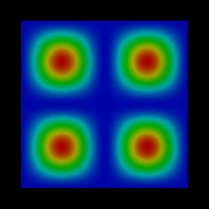
Figure 2.4.549 Probability density
Note that these wave functions were obtained by using a single-band effective mass approximation for the holes. A more accurate and more realistic treatment would have been to use 6-band k.p. Note that the wire has been assumed to be unstrained (which is a rather unphysical situation) for the purpose to make this tutorial easier to understand.
Hole wave functions (with magnetic field)
To include the magnetic field in the simulation, the variable $magnetic_field_on should be set to 1 in the input file. Here, we assume a field strength of 1 T.
$magnetic_field_on       = 1      # choose 1 (magnetic field on) or 0 (magnetic field off)
$magnetic_field_strength = 1.0    # Strength of the magnetic field [T]
The
database{
    binary_zb {
        name = InAs
        valence_bands{
            HH{ mass = 0.41  g = 0}
        }
    }
}
In the following figures the probability densities
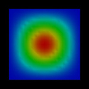
Figure 2.4.550 Probability density
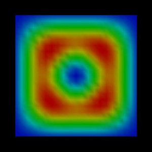
Figure 2.4.551 Probability density

Figure 2.4.552 Probability density
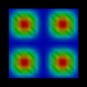
Figure 2.4.553 Probability density
In Figure 2.4.554, the probability density of the
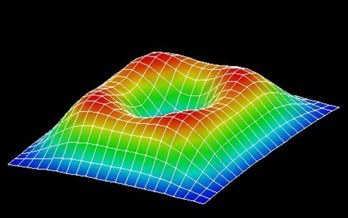
Figure 2.4.554 Probability density
6-band k.p approximation
The corresponding input file is QWR-magnetic-field_InAs_2D_6kp_nnp.in. Here, we used the following Dresselhaus parameters for InAs:
Hole wave functions - (without magnetic field)
The following figures show the probabilities densities
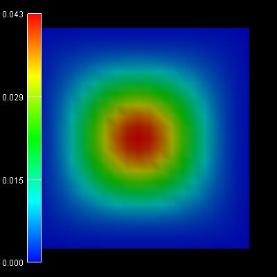
Figure 2.4.555 Probability density of the

Figure 2.4.556 Probability density of the
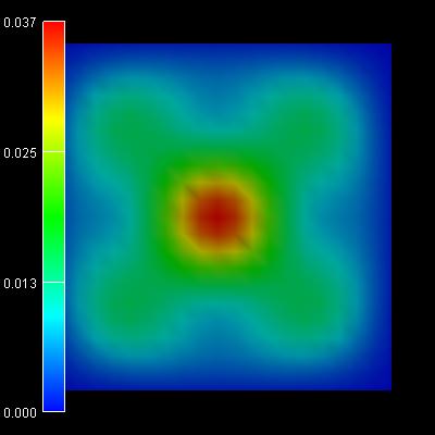
Figure 2.4.557 Probability density of the

Figure 2.4.558 Probability density of the
Last update: nnnn/nn/nn