— EDU — Orbitals of the Hydrogen Atom

Header

Files for the tutorial located in nextnano++\examples\education

• Orbitals_Hydrogen_3D_nnp.in

Scope of the tutorial:

• Schrödinger equation

• Coulomb potential

• Numerical accuracy

Main adjustable parameters in the input file:

• regularizing parameter $eta

• radius of the simulation domain $pos_end

• positions of the grid definitions: $pos_fine, $pos_medium, and $pos_coarse

• grid spacings: $grid_coarse, $grid_medium, and $grid_fine

Relevant output files:

• bias_00000\bandedge_Gamma_1d_z.dat

• bias_00000\bandedge_Gamma_2d_yz.dat

• bias_00000\Quantum\energy_spectrum_quantum_region_Gamma_00000.dat

• bias_00000\Quantum\amplitude_quantum_region_Gamma_XXXX.fld

Introduction

This tutorial demonstrates use of nextnano++ in computing orbitals of a Hydrogen atom. As orbitals and their energies can be obtained analytically for the Hydrogen atom (see. [LeviAQM2006]), this tutorial serves also as a playground for exploration of numerical limits of 3D simulations on small computers.

In this tutorial we assume that the proton is set in the origin of the coordinate system and the electron is confined by the Coulomb potential arising from the presence of the proton

(2.4.39)$${\varphi }_C(r)=\frac{1}{4\pi {\epsilon }_0}\frac{q}{r},$$

where $q$ is the elementary charge, $r$ is a distance from the proton, and ${\epsilon }_0$ is the permittivity of vacuum. This potential can be defined directly in the input file using coordinates as

$$r=\sqrt{x^2+y^2+z^2}$$

Note that the length is given in (nm) in the input file. The Schrödinger equation for the system is given by

(2.4.40)$$[-\frac{{\hslash }^2}{2m_0}{\mathrm{\nabla }}^2-q{\varphi }_C(x,y,z)]\mathrm{\Psi }(x,y,z)=E\mathrm{\Psi }(x,y,z),$$

where $m_0$ is the mass of a free electron and $\hslash$ is Dirac’s constant.

This equation can be solved by nextnano++ within 1-band model. To do so one needs to take care about:

• definition of a convenient vacuum “material”,

• grid spacing and size of the simulation domain,

• infinity of the potential at the origin of the coordinate system.

Preparing the simulation

Convenient vacuum “material”

Let us define vacuum material modifying existing material, e.g., GaAs. As energy dispersion of electron in vacuum is isotropic parabola, 1-band model for conduction band for zincblende crystals can be parametrized to describe vacuum. The effective mass corresponding to the free electron is equal to 1. Assuming that total energy of stationary electron is equal 0 eV, we set the minimum of the band to be zero. We do it safely by setting all: band gap, band offset, and spin-orbit splitting to zero.

database{ # gallium arsenide turned into vacuum at 0 eV
    binary_zb{
        name = GaAs # same as the substrate to neglect strain
        conduction_bands{
            Gamma{
                bandgap = 0
                mass    = 1
            }
        }
        valence_bands{
            bandoffset = 0
            delta_SO = 0
        }
    }
}

Note that we also turn off temperature dependence of the band gap so that Varshi formula is not applied and does not shift the minimum. Choice of the crystal orientation and substrate are arbitrary in this simulation. We set some, because the solver requires them. All strain effects are ignored as strain{ } is not called in the run{ } section - there is no strain in the vacuum.

global{
    simulate3D{}
    crystal_zb{
        x_hkl = [1, 0, 0]
        y_hkl = [0, 1, 0]
    }
    substrate{ name = "GaAs" }

    temperature_dependent_bandgap = no
    temperature = 4.0 # Kelvin
}

The vacuum is ready!

The grid and simulation domain

Keeping in mind that these computations are meant to be held on desktop computers or laptops, the biggest limitation comes from the number of grid points that one can include in the simulation, as it directly impacts RAM needed for the simulation. The simulation grid should be defined to have possibly low number of grid points while keeping most of them the center of the atom to properly represent the potential and orbitals of interest.

In the input file for this tutorial we defined such a grid to keep it fine nearby the center of the atom and gradually coarser while going outwards (basic example on how to define such grids can be found here). For that purpose we use 6 variables to have quite flexible control over the grid spacing ($grid_coarse, $grid_medium, and $grid_fine) and positions where these spacings begin to apply ($pos_fine, $pos_medium, and $pos_coarse). The last parameter of the grid, $pos_end, is defining the size of the entire simulation domain.

All of these parameters together are determining number of grid points, hence, how much memory the simulation will require and how much time it will take to have the Schrödinger equation solved.

   #spacing
   $grid_coarse = 0.1
   $grid_medium = 0.05
   $grid_fine = 0.005

  grid{
      xgrid{
         line{ pos =-$pos_end       spacing = $grid_coarse }
         line{ pos =-$pos_coarse    spacing = $grid_coarse }
         line{ pos =-$pos_medium    spacing = $grid_medium }
         line{ pos =-$pos_fine      spacing = $grid_fine   }
         line{ pos = 0              spacing = $grid_fine   }
         line{ pos = $pos_fine      spacing = $grid_fine   }
         line{ pos = $pos_medium    spacing = $grid_medium }
         line{ pos = $pos_coarse    spacing = $grid_coarse }
         line{ pos = $pos_end       spacing = $grid_coarse }
        }
      ygrid{
          line{ pos =-$pos_end      spacing = $grid_coarse }
         line{ pos =-$pos_coarse    spacing = $grid_coarse }
         line{ pos =-$pos_medium    spacing = $grid_medium }
         line{ pos =-$pos_fine      spacing = $grid_fine   }
         line{ pos = 0              spacing = $grid_fine   }
         line{ pos = $pos_fine      spacing = $grid_fine   }
         line{ pos = $pos_medium    spacing = $grid_medium }
         line{ pos = $pos_coarse    spacing = $grid_coarse }
         line{ pos = $pos_end       spacing = $grid_coarse }
        }
      zgrid{
         line{ pos =-$pos_end       spacing = $grid_coarse }
         line{ pos =-$pos_coarse    spacing = $grid_coarse }
         line{ pos =-$pos_medium    spacing = $grid_medium }
         line{ pos =-$pos_fine      spacing = $grid_fine   }
         line{ pos = 0              spacing = $grid_fine   }
         line{ pos = $pos_fine      spacing = $grid_fine   }
         line{ pos = $pos_medium    spacing = $grid_medium }
         line{ pos = $pos_coarse    spacing = $grid_coarse }
         line{ pos = $pos_end       spacing = $grid_coarse }
        }
    }

Note

In general, the accuracy increases with reduction of the grid, unless machine precision begins to limit accuracy of derivatives.

Regularized Coulomb potential

The Coulomb potential itself is posing a problem in this simulation as it introduces infinity, which gets more and more severe when the grid gets finer around it. One way to remove this infinity is to regularize the potential (2.4.39) introducing a regularizing parameter $\eta$ aiming at removing the infinity.

(2.4.41)$${\varphi }_C(r)\to {\varphi }_{\eta }(r)=\frac{1}{4\pi {\epsilon }_0}\frac{q}{\sqrt{x^2+y^2+z^2+{\eta }^2}}$$

Assuming that one cares about accuracy for the ground state in the Hydrogen atom, the $\eta$ should not modify the potential much outside a volume that is negligibly small in comparison to the orbital 1s. Otherwise the regularization will notably affect eigenenergy and shape of this orbital. We chose $\eta =3.5\cdot {10}^{-3}$ nm, which is around one order of magnitude smaller than the Bohr radius, $a_B\approx 5.3\cdot {10}^{-2}$ nm.

This potential we define inside the import{ } group using $eta (see top of the input file) as a variable corresponding to $\eta$.

$e = 1 #eV
$eps = 55.263E-3 #e^2eV^(-1)nm^(-1)
$pi = 3.1415

import{
    analytic_function{
        name = "Potential"
        function = "(1/(4*$eps*$pi))*( $e/(sqrt((x)^2 + (y)^2 + (z)^2 + $eta^2)) )"
        label = potential_label
    }
output_imports{}   # output all imported data including scale factor.
}

The potential is included as an initialization of Poisson equation, which further is not solved.

   poisson{
      import_potential{ import_from = "Potential" }
      output_potential{}
    }

Results and Discussion

Orbitals s1 and s2

Let us have a look at s orbitals that are expected to be the most affected by regularization of the Coulomb potential. One can easily compare these orbitals with literature [LeviAQM2006] as their amplitudes have symmetry of a sphere. To do so, one can define 1D sections through the center of the atom in the input file using section{ } nested group and plot numerical amplitudes together with the ones derived analytically

(2.4.42)$$\begin{array}{r}\begin{array}{rl}{\mathrm{\Psi }}_{1s}(r)& =2{\left(\frac{1}{a_B}\right)}^{3/2}\exp (-\frac{r}{a_B}){\left(\frac{1}{4\pi }\right)}^{1/2},\\ {\mathrm{\Psi }}_{2s}(r)& =2{\left(\frac{1}{2a_B}\right)}^{3/2}(1-\frac{r}{2a_B})\exp (-\frac{r}{2a_B}){\left(\frac{1}{4\pi }\right)}^{1/2}.\end{array}\end{array}$$

Such comparison of s1 and s2 orbitals obtained with both methods is shown in Figure 2.4.127 a) and b), respectively.

Figure 2.4.127 a), b) Comparison of 1s and 2s orbitals obtained from analytical formulas and numerical simulation. c), d) Difference between the analytical and numerical wave functions of s1 and s2 orbitals, respectively.

As seen in the Figure 2.4.127 c) and d), the most significant loss of accuracy is present near the center of the atom, where regularization has the biggest effect. It reaches approximately 10% of the maximum amplitude at the zero coordinate, and falls below 1% at radius smaller than 0.05 nm.

Regularized potential

Investigating the potential (see Figure 2.4.128) one can see that regularization impacts the potential in the order of magnitude 10^-2 - 10^-1 V at the distance near the Bohr radius.

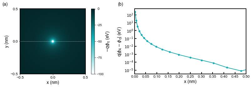
Figure 2.4.128 (a) shows the Coulomb energy distribution. (b) is the difference between the numerical Coulomb potential $(V_{\eta })$ calculated by nextnano++ and the analytical potential $(V_A)$ at $y=0$, $z=0$ along the white dash line in (a).

For that reason, a well-computed first orbital can be expected to have the eigenenergy deviating from the analytical value by approximately 10^-2 - 10^-1 eV.

Energies

Accordingly, the effect can be best seen by comparing analytical energies of orbitals [LeviAQM2006]

(2.4.43)$$E_a=\frac{-m_0{q}^4}{2(4\pi {\epsilon }_0{)}^2{\hslash }^2}\frac{1}{n^2},$$

where $n$ is the principal quantum number, with computation using a fine grid ($grid_medium=0.01); see columns 4-6 in Table 2.4.1. Here the difference of energies is overestimated by approximately 0.19 eV for the ground state, which corresponds to additional potential energy introduced by the regularization.

Table 2.4.1 Eigenenergies obtained using analytical formula ($E_a$), from the simulation with fine grid ($E_{fine}$) and coarser grid ($E_{fine}$) to reduce simulation time.

$Orbital$	$n$	$l$	$E_a$ (eV) (*)	$E_{fine}$ (eV)	$|E_{fine}-E_a|$ (eV)	$E_{fast}$ (eV)	$|E_{fast}-E_a|$ (eV)
$1s$	$1$	$0$	$-13.606$	$-13.420$	$1.86\times {10}^{-2}$	$-13.605$	$1.26\times {10}^{-3}$
$2s$	$2$	$0$	$-3.401$	$-3.381$	$1.96\times {10}^{-2}$	$-3.424$	$2.25\times {10}^{-3}$
$2p$	$2$	$1$	$-3.401$	$-3.402$	$1.44\times {10}^{-3}$	$-3.450$	$4.85\times {10}^{-2}$
$2p$	$2$	$1$	$-3.401$	$-3.402$	$1.44\times {10}^{-3}$	$-3.450$	$4.85\times {10}^{-2}$
$2p$	$2$	$1$	$-3.401$	$-3.402$	$1.44\times {10}^{-3}$	$-3.450$	$4.85\times {10}^{-2}$
$3s$	$3$	$0$	$-1.512$	$-1.506$	$5.81\times {10}^{-3}$	$-1.525$	$1.34\times {10}^{-2}$
$3p$	$3$	$1$	$-1.512$	$-1.512$	$4.40\times {10}^{-4}$	$-1.532$	$1.96\times {10}^{-2}$
$3p$	$3$	$1$	$-1.512$	$-1.512$	$4.40\times {10}^{-4}$	$-1.532$	$1.96\times {10}^{-2}$
$3p$	$3$	$1$	$-1.512$	$-1.512$	$4.40\times {10}^{-4}$	$-1.532$	$1.96\times {10}^{-2}$
$3d$	$3$	$2$	$-1.512$	$-1.513$	$5.49\times {10}^{-4}$	$-1.528$	$1.63\times {10}^{-2}$
$3d$	$3$	$2$	$-1.512$	$-1.513$	$5.49\times {10}^{-4}$	$-1.528$	$1.63\times {10}^{-2}$
$3d$	$3$	$2$	$-1.512$	$-1.512$	$3.92\times {10}^{-5}$	$-1.521$	$8.91\times {10}^{-3}$
$3d$	$3$	$2$	$-1.512$	$-1.512$	$3.92\times {10}^{-5}$	$-1.521$	$8.91\times {10}^{-3}$
$3d$	$3$	$2$	$-1.512$	$-1.512$	$3.92\times {10}^{-5}$	$-1.521$	$8.91\times {10}^{-3}$

Such fine simulation, however, can take more than half a day to finish. Interesting results can be also obtained using coarser grid, therefore, within shorter simulation runs (couple of minutes). Columns 4 and 7-8 of Table 2.4.1 show that it is possible to match energy of the first orbital with the analytical results. However, this is just a luck arising from lowering of numerical accuracy due to coarser grid. The proof are energies of all further orbitals, which deviate from analytical solutions much more than for the fine simulation, moreover, being reduced instead of increased despite additional energy introduced by regularization. As expected, the discrepancy is further gradually reducing as orbitals are localized further away from the center of the potential; amplitudes are less varying in space. The choice of the grid, therefore, depends on the goal of the simulation and must be performed carefully.

Degeneracy of orbitals

Finally, let us have a look at selected amplitudes of orbitals in the Hydrogen atom shown in Figure 2.4.129.

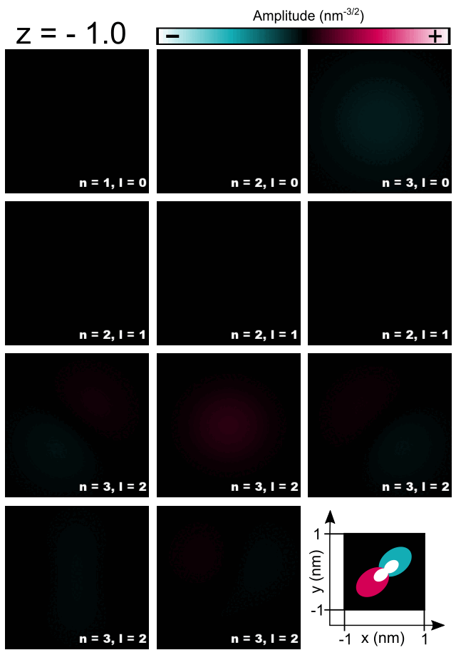
Figure 2.4.129 Cross-sections of 1s, 2s, 3s, 2p, and 3d orbitals computed for the Hydrogen atom.

As the energy of the orbital without presence of magnetic field is given only by the principal quantum number $n$ one should expect that all computed orbitals within one shell will be randomly superposed. For those, who do not look for such effects, fortunately, symmetry of numerical grid and regularization are partly breaking this degeneracy and the orbitals are distinguishable to some degree. All three orbitals 1s, 2s, 3s may have additionally overestimated energy due to regularization which makes them always separated from superposing with other orbitals; grid may have its own effect here as well. Orbitals p seems to have different energies from orbitals d due to symmetry of the grid influencing their energies as these orbitals have different value of the azimuthal quantum number $l$. The three orbitals 2p do not look exactly like in the books; they are tilted but seem to have proper relative orientation. The orbitals 3d seems to be notably superposed, however, they remain recognizable and similar to the orbitals shown in the literature. Because the numerical results tend to be rotated and superposed to some degree, the magnetic quantum number is not easy to be indicated and ommited in the Figure 2.4.129 and the Table 2.4.1.

Exercises

Compute lowest s, p, and d orbitals of a hydrogen atom and answer following questions:

• Are computed wave-functions of s orbitals in agreement with analytical solutions?

• Are all energies of orbitals the same as obtained analytically? If not, why do they deviate from analytical solutions?

• Is proper degeneracy present in the numerical solutions?

Additional question on numerics:

• What is the biggest regularizing parameter that can be used for the electrostatic potential and grid spacing if one aims at 1 meV accuracy for the energy of the ground state?

---

Last update: 27/10/2023