| nextnano.com nextnano³ Download | Search | Copyright | Publications * password protected |
nextnano³ software
|
|
| BIO-1D Protein sensor |
|
|
|
|
|
nextnano3 - Tutorialnext generation 3D nano device simulator1D TutorialISFET (Ion-Selective Field Effect Transistor): Detection of charged proteins with a SOI (silicon-on-insulator) electrolyte sensorAuthor: Stefan Birner If you want to obtain the input file that is used within this tutorial, please
submit a support ticket. ISFET (Ion-Selective Field Effect Transistor): Detection of charged proteins with a SOI (silicon-on-insulator) electrolyte sensorThis tutorial is based on the following paper:
The general idea of this paper has been presented already in the diploma thesis of Christian Uhl, Charge Transport at Functionalized Semiconductor Surfaces, TU Munich (2004). The simulations are based on previously performed experiments:
Summary For a bio-sensor device based on a silicon-on-insulator (SOI) structure, we calculate the sensitivity to specific charge distributions in the electrolyte solution that arise from protein binding to the semiconductor surface. This surface is bio-functionalized with a lipid layer so that proteins can specifically bind to the headgroups of the lipids on the surface. We consider charged proteins such as the green fluorescent protein (GFP) and artificial proteins that consist of a variable number of aspartic acids. Specifically, we calculate self-consistently the spatial charge and electrostatic potential distributions for different ion concentrations in the electrolyte. We fully take into account the quantum mechanical charge density in the semiconductor. We determine the potential change at the binding sites as a function of the protein charge and ionic strength. Comparison with experiment is generally very good. Furthermore, we demonstrate the superiority of the full Poisson-Boltzmann equation by comparing its results to the simplified Debye-Hückel approximation.
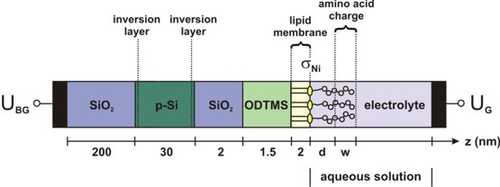
We discuss a silicon-on-insulator (SOI) based thin-film resistor that we will model in detail in this tutorial. Indeed, such a device has been realized experimentally for chemical and biological sensor applications. Peptides with a single charge can be detected and it is possible to distinguish single charge variations of the analytes even in physiological electrolyte solutions. Figure 1 shows the layout of this bio-functionalized silicon-on-insulator device. It consists of a SiO2-Si-SiO2 structure. Specifically, we take a silicon dioxide buffer layer with a thickness of 200 nm (0 nm - 200 nm) and a conducting silicon layer of 30 nm (200 nm - 230 nm) which is homogeneously p-type doped with boron (doping density p = 1 * 1016 cm-3). The silicon layer is covered by a native SiO2 layer with a thickness of 2 nm (230 nm - 232 nm).
This oxide layer is passivated by an ODTMS (octadecyltrimethoxysilane) monolayer which is required for the bio-functionalization of the semiconductor device. We take a 1.5 nm thick oxide-like ODTMS layer (232 nm - 233.5 nm) and use a static dielectric constant of epsilon = 1.5. Due to the passivation by ODTMS, we assume that no interface charges are present at the native oxide surface. The ODTMS layer is surface-functionalized with a lipid membrane that allows the specific binding of molecules. This lipid monolayer (2 nm) consists of DOGS-NTA (1,2-dioleoyl-sn-glycero-3-{[N(5-amino-1-carboxypentyl)iminodiacetic acid]succinyl}) incorporated into two matrix lipids (DMPC (1,2-dimyristoyl-sn-glycero-3-phosphocholine) and cholesterol). The lipid membrane is treated as an insulator using the same material parameters as for ODTMS. Thus, no charge carriers are assumed to be present within this layer. As the lipid layer is very dense, no electrolyte is considered within the lipid region. The functionalized surface exposes NTA headgroups that carry two negative charges to the electrolyte solution. They have the ability to form a chelate complex with nickel ions if the latter are present in the solution. Upon loading with nickel, the charge of the headgroup changes by +1e and is then considered to be -1e. This results in a negative sheet density sigmaNi at the lipid/electrolyte interface. The surface density of the DOGS-NTA lipids is considered to be 5 % (fNTA = 0.05). The approximated headgroup area, i.e. the average area per functional DOGS-NTA is assumed to be ANTA = 0.65 nm2. Consequently, the density of the headgroups is sNTA = fNTA / ANTA = 7.7 * 1012 cm-2, so that the resulting charge density sigmaNi is given by sigmaNi = - e * sNTA, where we have assumed that each headgroup carries one negative charge upon exposure to Ni.
For the ionic content of the electrolyte we consider a variable concentration of KCl (i.e. 10, 50, 90 or 140 mM), and a fixed concentration of 1 mM NiCl2 and 1 mM of phosphate buffer saline (PBS) solution, respectively. The NiCl2 dissociates into 1 mM of doubly charged cations and 2 mM of singly charged anions. For all calculations, the pH of the bulk electrolyte has been set to 7.5.
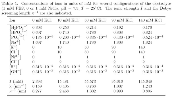
The calculated concentrations of the PBS buffer ions are listed in Table 1 for different salt concentrations. These values refer to the bulk electrolyte. In the vicinity of the semiconductor surface and in regions around charged analytes, however, the actual concentrations of the buffer ions vary locally. Our buffer model automatically takes this into account because the spatial variations of pH, ionic strength and pKa,T' are determined self-consistently (see Appendix B of the above mentioned paper for more details). The ionic strengths of the electrolyte solutions considered in this work, are largely dominated by the respective concentrations of singly charged anions and cations from KCl as can be seen in Table 1. In these particular cases, i.e. small concentrations of PBS with respect to KCl, the Debye screening length is fully dominated by the KCl concentration.
The electrolyte region (235.5 nm - 999 nm) contains the following ions (plus
the buffer ions!): In addition to these four types of ions, the pH value (as specified in
In addition to the previously described ions, additional ions occur due to the buffer. Here, a PBS buffer (phosphate buffer) is used with a concentration of 1 mM. We calculate the concentration of the buffer ions automatically depending on temperature, ionic strength, pH value, pKa,T' value(s) and spatial coordinate. For that reason, four additional types of ions are present: H2PO4
Electrode potential UGIn order to allow for comparison with experiment, we need to determine the potential of the reference electrode in the electrolyte. We consider a SOI structure that is operated in inversion. This means that the p-doped Si channel is inverted and becomes n-type. The electrode in the solution is assumed to determine the bulk electrolyte potential UG. In this example the applied gate voltage is UG = 2.2 V. This value yields channel densities of the order of a few 1011 cm-2 depending on the actual configuration of the system in terms of ion concentrations and protein charges. The experiment also yields electron densities of this magnitude. We note that the electrode potential UG does not reflect the experimentally applied potential since we do not take into account potential drops at the electrode. UG is defined on a scale where the Fermi energy in the semiconductor determines zero potential. We have to solve the nonlinear Poisson equation over the whole device, i.e.
including the Poisson-Boltzmann equation that governs the charge density in the
electrolyte region. We simulate the structure along the z direction
so that the structure is effectively
one-dimensional, i.e. laterally homogeneous. Protein charge distributionWe study a protein charge distribution that is
spatially separated from the lipid membrane due to a neutral tag in between the
protein and the lipids. The protein is modeled to allow for comparison with
experiment. We consider an artificial protein structure where amino acids are
tagged to a histidine chain. A part of this artificial protein remains uncharged
since no amino acids get attached there. The width of this part has been taken
to be 1.5 nm. By contrast, the rest of the histidine backbone is negatively
charged since we consider aspartic acids (ASP) that carry one negative charge
each for the binding to the tag. The electrolyte region starts at the membrane
surface and includes the regions of both the neutral part of the tag and the
protein charge distribution so that the ions in the aqueous solution screen the
protein charge. Fig. 1 illustrates the structure as considered for the
calculations. The artificial protein binds to an NTA headgroup on the membrane.
It is possible to manufacture the protein consisting of his-tagged aspartic
acids (ASP) that bind to the tag. The integrated charge density in the protein
region therefore changes in magnitudes of We represent the aspartic acids by a doping function.
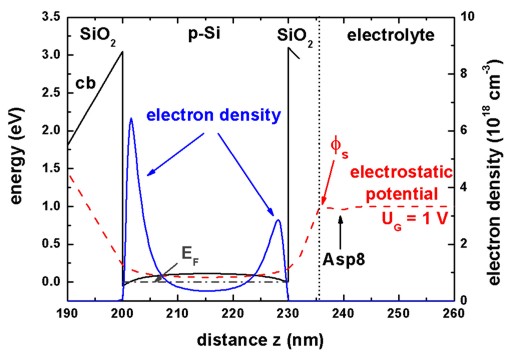
Conduction band edge and electron densitySince we have specified all about the sensor and the proteins in the electrolyte, we are now ready to calculate the electrostatic potential in the semiconductor/electrolyte system for several protein charge distributions. The quantum mechanical charge densities are calculated self-consistently by solving the Schrödinger equation in the silicon channel. The Schrödinger and Poisson equations are coupled via the electrostatic potential and the charge densities. Figure 2 shows the calculated conduction band
edge and the electron density in the
silicon channel for a backgate voltage of UBG = 25 V. Indicated is
also the position of the Fermi level EF and the
electrostatic potential. Specifying a value for
the potential UG of the reference electrode is equivalent to a
Dirichlet boundary condition for the electrostatic potential of the
Poisson-Boltzmann equation. An increase of UG leads to higher
electron densities in the right channel. Therefore, the variation of UG
and the backgate voltage UBG allows one to increase the sensitivity
of the sensor by adjusting the ratio of the densities of the two channels. Our
calculations yield channel densities of the order of a few 1012 cm
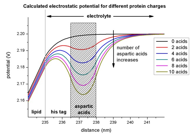
Electrostatic potential for different numbers of aspartic acidsWe calculated the potential and charge distributions in the semiconductor/electrolyte structure self-consistently for different numbers of aspartic acids. Importantly, variations of the protein charge distribution that affect the potential in the SOI structure are calculated. Since the potential at the lipid/electrolyte interface sets the boundary value for the spatial potential distribution in the semiconductor, we determine the lipid/electrolyte interface potential and its changes as a function of the respective parameter that is varied. The interface potential is also referred to as the surface potential since the lipid layer constitutes the surface of the semiconductor. The magnitude of the negative protein charge density increases with the number of aspartic acids. This results in a lower potential in the protein region. Fig. 3 shows the calculated potential distribution for a varying number of aspartic acids where the surface potential decreases with increasing protein charge. The pH value of the electrolyte has been set to 7.5 and the concentration of KCl in the solution has been assumed to be 140 mM. As already mentioned, the neutral part of the histidine tag is assumed to be 1.5 nm. The respective protein charges that are considered have been homogeneously distributed over 1.5 nm and are indicated by the shaded region in Fig. 3. We have considered the chemical structure of the histidine tagged amino acids in order to obtain this parameter. We note, that the electrolyte region starts at the lipid surface at 236 nm. Now we want to plot the electrostatic potential for different numbers of aspartic acids.
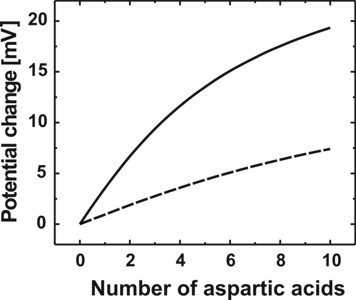
Surface potential changeWe calculated the potential change at the lipid membrane as a function of the number of aspartic acids that are attached to each histidine tag for KCl concentrations of 50 mM and 140 mM. The reference level phiref,surface for the surface potential change scale is the one for zero protein charge. We define the surface potential change Delta_phi by
where NASP denotes the number of aspartic acids. A positive potential
change therefore implies that the reference level is higher compared to the
situation with a nonzero number of aspartic acids. The results are shown in Fig.
4. Due to the lower ion concentrations in the case of 50 mM KCl, the protein
charge density is less efficiently screened. Consequently, the surface potential
change is larger compared to the case of 140 mM KCl. Therefore the variations in
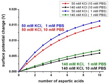
the charge density in the silicon channel are greater in the case of 50 mM KCl. The right figure shows the different sensitivity due to the PBS buffer concentrations. Using a 1 mM PBS buffer reduces the ionic strength and thus the screening of the aspartic acid charges with respect to the 10 mM PBS buffer.
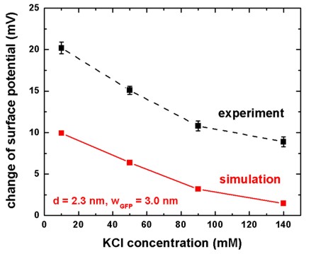
Influence of the ionic strength on the sensitivityGreen fluorescent proteinAs a second protein, we consider the binding of the so-called green fluorescent protein (GFP) to the lipid membrane. GFP is also histidine-tagged to the NTA headgroups of the membrane. The size of GFP is larger (length of 4-5 nm) compared to his-tagged aspartic acids. We assume a charge distribution of width w = 3.0 nm that is connected with a neutral tag of width d = 2.3 nm to the NTA headgroups. At pH = 7.5, GFP carries eight negative charges that we assume to be homogeneously distributed over the protein region w. Here, we use the same sensor structure as in Fig. 1 but detect another protein. We consider the specific binding of the green fluorescent protein (GFP) to the lipid membrane and calculate the change of the surface potential as a function of the salt concentration (10, 50, 90 or 140 mM KCl) in the electrolyte. At pH = 7.5, GFP carries a net negative charge of -8e as can be derived from the primary structure if one calculates the charge of the sidechains for the used buffer solution. Consequently, the integrated charge density of GFP is given by sigmaGFP = - 8 e sNTA. We assume for simplicity that this charge is distributed evenly over a distance of wGFP = 3 nm which is close to the length of the GFP (4-5 nm). Based on the previous section, the length of the neutral part of the tag has been taken to be d = 2.3 nm. Here, this length has been assumed to be the same for all KCl concentrations.
We have calculated the change of the surface potential as a function of the
KCl concentration in the electrolyte. The electrolyte has the same properties as
for the aspartic acids (1 mM PBS, 1 mM NiCl2). Figure 5 shows the
results and compares them to the experimental data of the above cited reference.
The trend of the influence of the ionic strength on the sensitivity is well
reproduced by our calculations. We note that the exact orientation of the GFP
molecule at the surface is not known. A slight tilt angle can increase the
measured sensor response due to the exponential dependence of the signal from
the distance of the charges. The reduction of the spacing d or the |
|
|