k.p dispersion in bulk GaAs (strained / unstrained)

Input files:

• bulk_kp_dispersion_GaAs_nnp.in

• bulk_kp_dispersion_GaAs_nnp_strained.in

Scope:

We calculate $E(k)$ of strained and unstrained $GaAs$.

Band structure of bulk $GaAs$

Input file: bulk_kp_dispersion_GaAs_nnp.in

We want to calculate the dispersion $E(k)$ from $|k|$ = 0 nm^-1 to $|k|$ = 1.0 nm^-1 along the following directions in k space:

• [000] to [110]

• [000] to [100]

We compare 6-band and 8-band k.p theory results. We calculate $E(k)$ for bulk $GaAs$ at a temperature of 300 K.

Bulk dispersion along [100] and along [110]

quantum{
    region{
        ...
        bulk_dispersion{
            lines{ # set of dispersion lines along crystal directions of high symmetry
                name = "lines"
                position{ x = 5.0 }
                k_max = 1.0
                spacing  = 0.01
                shift_holes_to_zero = yes
            }

            path{ # dispersion along arbitrary path in k-space
                name = "user_defined_path"
                position{ x = 5.0 }
                point{ k = [0.7071, 0.7071, 0.0] }
                point{ k = [0.0, 0.0, 0.0] }
                point{ k = [1.0, 0.0, 0.0] }
                spacing  = 0.01
                shift_holes_to_zero = yes
            }
        }
    }
}

We calculate the pure bulk dispersion at position x = 5 nm. In our case this is $GaAs$, but it could be any strained alloy. In the latter case, the k.p Bir-Pikus strain Hamiltonian will be diagonalized. The grid point at position{ x = 5.0 } must be located inside a quantum region. shift_holes_to_zero = yes forces the top of the valence band to be located at 0 eV. How often the bulk k.p Hamiltonian should be solved can be specified via spacing. To increase the resolution, just increase this number. We use two direction in k space, i.e. from [000] to [110] and from [000] to [100]. In the latter case the maximum value of $|k|$ is

$$k_{\max }=\sqrt{{0.7071}^2+{0.7071}^2}=1.0$$

Note that for values of $|k|$ larger than 1.0 nm^-1, k.p theory might not be a good approximation anymore.

The results of the calculation can be found in the folder bias_00000\Quantum\Bulk_dispersions. Figure 2.4.232 visualizes the results.

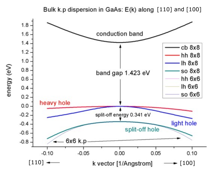
Figure 2.4.232 Bulk k.p dispersion in $GaAs$: $E(k)$ along [100] and [110].

The split-off energy of 0.341 eV is identical to the split-off energy as defined in the database:

...
valence_bands{ delta_SO = 0.341 } # [eV] Vurgaftman1
...

If one zooms into the holes and compares 6-band vs. 8-band k.p, one can see that 6-band and 8-band coincide for $|k|$ < 1.0 nm^-1 for the heavy and light hole but differ for the split-off hole at larger $|k|$ values, see Figure 2.4.233.

Figure 2.4.233 Bulk k.p dispersion in GaAs: $E(k)$ along [100] and [110] - Comparision between 6x6 and 8x8 k.p

8-band k.p vs. effective-mass approximation

Now we want to compare the 8-band k.p dispersion with the effective-mass approximation. The effective mass approximation is a simple parabolic dispersion which is isotropic (i.e. no dependence on the k vector direction). For low values of k ($|k|$ < 0.4 nm^-1) it is in good agreement with k.p theory, see Figure 2.4.234.

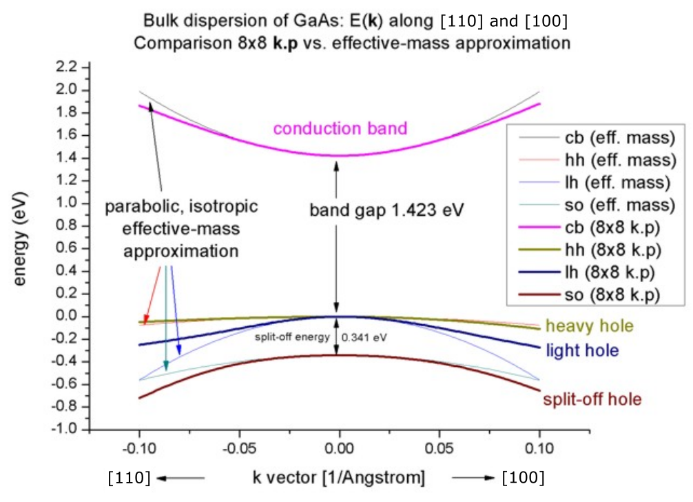
Figure 2.4.234 Bulk k.p dispersion in $GaAs$: $E(k)$ along [100] and [110] - Comparision between 8x8 k.p and effective-mass approximation

Band structure of strained $GaAs$

Input file: bulk_kp_dispersion_GaAs_nnp_strained.in

Now we perform these calculations again for $GaAs$ that is strained with respect to $I{n}_{0.2}G{a}_{0.8}As$. The $InGaAs$ lattice constant is larger than the $GaAs$ one, thus $GaAs$ is strained tensely. The changes that we have to make in the input file are the following:

strain{
    pseudomorphic_strain{ }
}

run{
    strain{ }
}

As substrate material we take $I{n}_{0.2}G{a}_{0.8}As$ and assume that $GaAs$ is strained pseudomorphically (pseudomorphic_strain{ }) with respect to this substrate, i.e. $GaAs$ is subject to a biaxial strain. Due to the positive hydrostatic strain (i.e. increase in volume or negative hydrostatic pressure) we obtain a reduced band gap with respect to the unstrained $GaAs$. Furthermore, the degeneracy of the heavy and light hole at $k‘=0islifted,see:numref:‘fig-1D-kp-dispersion-bulk-GaAs-kp-bandedges-strained$. Now, the anisotropy of the holes along the different directions [100] and [110] is very pronounced. There is even a band anti-crossing along [100]. (Actually, the anti-crossing looks like a “crossing” of the bands but if one zooms into it (not shown in this tutorial), one can easily see it.) Note: If biaxial strain is present, the directions along $x$, $y$ or $z$ are not equivalent anymore. This means that the dispersion is also different in these directions ([100], [010], [001]).

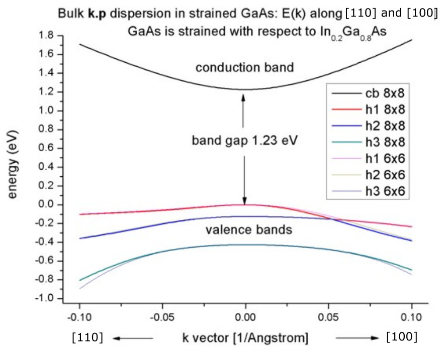
Figure 2.4.235 Bulk k.p dispersion in $GaAs$ strained with respect to $I{n}_{0.2}G{a}_{0.8}As$ : $E(k)$ along [100] and [110].

If one zooms into the holes and compares 6-band vs. 8-band k.p, one can see that the agreement between heavy and light holes is not as good as in the unstrained case where 6-band and 8-band k.p lead to almost identical dispersions, compare Figure 2.4.236.

Figure 2.4.236 Bulk valence band k.p dispersion in $GaAs$ strained with respect to $I{n}_{0.2}G{a}_{0.8}As$ : $E(k)$ along [100] and [110] - Comparision between 6x6 and 8x8 k.p approximation.

Note that in the strained case, the effective-mass approximation is very poor.

Analysis of eigenvectors

(preliminary)

Using the Voon-Willatzen-Bastard-Foreman k.p basis one obtains the following output for the eigenvectors at the Gamma point, $k$ = ($k_x$, $k_y$, $k_z$) = 0.

Example: The x_up component contains a complex number. Here, we show the square of X_up. This gives us information on the strength of the coupling of the mixed states.

   eigenvalue  S+     S-     HH     LH     LH     LH     SO     SO
1           0      1.0    0      0      0      0      0      0
2           1.0    0      0      0      0      0      0      0
3           0      0      0      1.0    0      0      0      0
4           0      0      0      0      1.0    0      0      0
5           0      0      0      0      0      1.0    0      0
6           0      0      1.0    0      0      0      0      0
7           0      0      0      0      0      0      0      1.0
8           0      0      0      0      0      0      1.0    0

eigenvalue  S+          S-          X+          Y+          Z+          X-          Y-          Z-
1           1.0         0           0           0           0           0           0           0
2           0           1.0         0           0           0           0           0           0
3           0           0           0           0           0.5         0.5         0           0
4           0           0           0           0           0.166       0.166       0.666       0
5           0           0           0.5         0           0           0           0           0.5
6           0           0           0.166       0.666       0           0           0           0.166
7           0           0           0           0           0.333       0.333       0.333       0
8           0           0           0.333       0.333       0           0           0           0.333

+: spin up, -: spin down

• The electron eigenstates are 2-fold degenerate, i.e. have the same energy, and are decoupled from the holes.

  1	$|S\downarrow ⟩$ $$
  2	$|S\uparrow ⟩$ $$

• The hole eigenstates are 4-fold (heavy and light holes) and 2-fold degenerate (split-off holes).

  3	$|\frac{3}{2},\frac{3}{2}⟩$ $$ hh spin up	$\frac{1}{\sqrt{2}}|(X+iY)\uparrow ⟩$
  4	$|\frac{3}{2},\frac{1}{2}⟩$ $$ lh	$\frac{1}{\sqrt{6}}|(X+iY)\downarrow ⟩-\sqrt{\frac{2}{3}}|Z\uparrow ⟩$
  5	$|\frac{3}{2},-\frac{1}{2}⟩$ $$ lh	$\frac{1}{\sqrt{6}}|(X-iY)\uparrow ⟩-\sqrt{\frac{2}{3}}|Z\downarrow ⟩$
  6	$|\frac{3}{2},-\frac{3}{2}⟩$ $$ hh spin down	$\frac{1}{\sqrt{2}}|(X-iY)\downarrow ⟩$
  7	$|\frac{1}{2},\frac{1}{2}⟩$ $$ s/o split	$\frac{1}{\sqrt{3}}|(X+iY)\downarrow ⟩-\frac{1}{\sqrt{3}}|Z\uparrow ⟩$
  8	$|\frac{1}{2},-\frac{1}{2}⟩$ $$ s/o split	$\frac{1}{\sqrt{3}}|(X-iY)\downarrow ⟩-\frac{1}{\sqrt{3}}|Z\downarrow ⟩$

  $\frac{1}{\sqrt{2}}$ = 0.707 $\to$ ${\left(\frac{1}{2}\right)}^2$ = 0.5

  $\frac{1}{\sqrt{3}}$ = 0.577 $\to$ ${\left(\frac{1}{3}\right)}^2$ = 0.333

  $\frac{1}{\sqrt{6}}$ = 0.408 $\to$ ${\left(\frac{1}{6}\right)}^2$ = 0.166

---

Last update: nn/nn/nnnn