— NEW — T-shaped quantum wire grown by cleaved edge overgrowth (CEO): wave functions without strain

Note

The tutorial is related to the PhD Thesis of R. Schuster [SchusterPhD2005]

Header

Input files:

• examples\quantum_wires\T-QWR_zb_III-V_Schuster_PhD_2005_2D_nnp.in

Scope:

Electron and hole wave functions of a T-shaped quantum wire (QWR).

Output files:

• \bias_xxxxx\Quantum\probabilities_quantum_region_Gamma.fld

• \bias_xxxxx\Quantum\probabilities_quantum_region_HH.fld

• \bias_xxxxx\Quantum\probabilities_quantum_region_LH.fld

• \bias_xxxxx\Quantum\probabilities_quantum_region_kp6_00000.fld

Structure

Similar to the 1D confinement in a quantum well, it is possible to confine electrons or holes in two dimensions, i.e. in a quantum wire. In this tutorial we consider the quantum wire, which is formed at the T-shaped intersection of two 10 nm $\mathrm{GaAs}$ type-I quantum wells, surrounded by ${\mathrm{Al}}_{0.35}{\mathrm{Ga}}_{0.65}\mathrm{As}$ barriers (see Figure 2.4.165). The electrons and holes are free to move along the $z$ direction only, thus the wire is oriented along the [0-11] direction. Such a heterostructure can be manufactured by growing the layers along two different growth directions with the CEO (cleaved egde overgrowth) technique. Due to the nearly identical lattice constants of GaAs and AlAs it is possible to assume this heterostructure as being unstrained.

The wave function is indicated at the T-shaped intersection in yellow. Here, the wave function can extend into a larger volume (as compared to the quantum well) and thus reduce its energy. Quantum mechanics tells us that the ground state can be found at this intersection and electrons are only allowed to move one-dimensionally along the $z$ direction. Figure 2.4.165 b) shows a 60 nm x 60 nm extract of the schematic layout including the dimensions, the material composition and the orientation of the wire with respect to the crystal coordinate system.

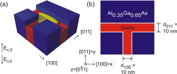
Figure 2.4.165 Two-dimensional conduction band edges of the T-shaped quantum wire.

Input file

It is sufficient to describe this heterostructure within a 2D simulation as it is translationally invariant along the $z$ direction. The simulation coordinate system is oriented in the following way:

global{
    simulate2D{}
    crystal_zb{
        x_hkl = [1, 0, 0]
        y_hkl = [0, 1, 1]
    }
}

As we do not have doping and no piezoelectric fields (the structure is assumed to be unstrained) and as the temperature is assumed to be 4 K, we do not have to deal with charge redistributions. Thus, we can refrain from solving Poisson’s equation, and we also do not have to take care about self-consistency.

Material parameters of relevance are the conduction band and valence band offset between $\mathrm{GaAs}$ and ${\mathrm{Al}}_{0.35}{\mathrm{Ga}}_{0.65}\mathrm{As}$:

$$\begin{array}{r}\begin{array}{c}\begin{array}{r}\\ \mathrm{CBO}& =0.2847\mathrm{eV}\\ \mathrm{VBO}& =-0.1926\mathrm{eV}\\ E_{\mathrm{gap},{\mathrm{Al}}_{0.35}{\mathrm{Ga}}_{0.65}\mathrm{As}}& =2.2883\mathrm{eV}\\ E_{\mathrm{gap},\mathrm{GaAs}}& =1.5193\mathrm{eV}\end{array}\end{array}\end{array}$$

Results

Using the input file T-QWR_GaAs-AlGaAs_Schuster_2005_2D_nnp.in we calculate the electron, heavy hole and light hole wavefunctions for the T-shaped quantum wire structure.

Effective mass approximation

The electron and hole wave functions can be calculated within the effective mass theory (envelope function approximation) by using position dependent effective masses. In our example, the effective masses are constant within each material but have discontinuities at the material interfaces. In nextnano++ the effective masses are assumed to be isotropic. Both, the heavy hole and the light hole band edge energies are degenerate but the effective masses differ. Thus, we have to solve three Schrödinger equations, namely for the conduction band, heavy hole band and light hole band. To trigger the 1-band effective mass model for calculating the eigenstates, use the following setting in the input file T-QWR_GaAs-AlGaAs_Schuster_2005_2D_nnp.in:

$kp6 = 0     # choose 1 (6 band k.p) or 0 (effective mass approximation) (ListOfValues: 1,0)

In Figure 2.4.166 we show the normalized probability densities (${\psi }^2$) for the electron, heavy hole and light hole ground states, which are obtained by the effective mass approximation.

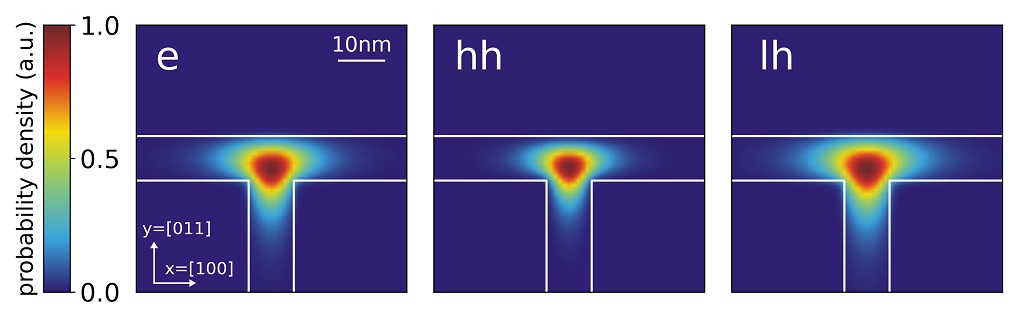
Figure 2.4.166 Probability densities of the electron (e), heavy hole (hh) and light hole (lh) state calculated using the effective mass approximation. The wavefunctions are normalized so that the maxima are equal to one.

In addition to these ground states for $k_z=0$, excited states are possible as well. Similar to the subbands of a 1D quantum well that show a $E(k_x,k_y)$ dispersion one can assign a subband with the energy dispersion $E(k_z)$ to each quantum wire eigenvalue which describes the free motion along the quantum wire axis ($z$ axis). A more advanced treatment would be to use k.p theory to calculate the eigenvalues for different $k_z$ in order to obtain the (nonparabolic) energy dispersion $E(k_z)$.

6-band k.p approximation

For the same structure as above we perform the calculations again, but this time using the 6-band k.p model instead of the single-band effective mass approximation. To trigger the 6-band k.p model for calculating the eigenstates, the following setting in the input file T-QWR_GaAs-AlGaAs_Schuster_2005_2D_nnp.in can be used:

$kp6 = 1     # choose 1 (6 band k.p) or 0 (effective mass approximation) (ListOfValues: 1,0)

Figure 2.4.167 shows the probability density (${\psi }^2$) for the hole ground state. For the results shown on the left we used the following Luttinger parameters for GaAs: ${\gamma }_1=6.98$, ${\gamma }_2=2.06$, ${\gamma }_3=2.93$, which corresponds to: $L=-16.220$, $M=-3.860$, $N=-17.580$. For the results shown on the right, we modified the Luttinger parameters for GaAs to ${\gamma }_1=6.98$, ${\gamma }_2=2.06={\gamma }_3$, which corresponds to $L=-16.220$, $M=-3.860$, $N=-12.36$. Choosing ${\gamma }_2={\gamma }_3$ corresponds to an isotropic effective mass.

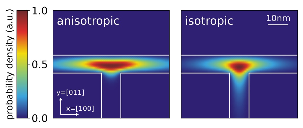
Figure 2.4.167 Probability density (${\psi }^2$) for the hole ground state using anisotropic and isotropic k.p parameters.

Eigenenergies

The calculated eigenvalues for the ground states are:

effective-mass			6-band k.p
electron energy (eV)	hh energy (eV)	lh energy (eV)	hole state energy (eV)
3.006	1.455	1.437	1.455

Including anisotropic effects in the effective mass model

Compared to nextnano++, nextnano³ allows using anisotropic effective masses for solving the Schrödinger equation within the effective mass approximation. The effective mass $m^{\ast }$ depends now on the chosen direction, which is described by a tensor. The components of the effective mass tensor, which are mass along the crystal coordinate axes, can be derived from the 6-band k.p parameters (or Luttinger parameters). Using the Luttinger parameters ${\gamma }_1$, ${\gamma }_2$ and ${\gamma }_3$, the effective masses for heavy and light holes along [110] and [010] in units of $m_0$ can be calculated as follows:

$$\begin{array}{r}\begin{array}{c}\begin{array}{r}\\ m_{\mathrm{hh},[100]}^{\ast }& =\frac{1}{{\gamma }_1-2{\gamma }_2},\\ m_{\mathrm{hh},[011]}^{\ast }& =\frac{1}{{\gamma }_1-0.5\cdot ({\gamma }_2+3{\gamma }_3)},\\ m_{\mathrm{lh},[100]}^{\ast }& =\frac{1}{{\gamma }_1+2{\gamma }_2},\\ m_{\mathrm{lh},[011]}^{\ast }& =\frac{1}{{\gamma }_1+0.5\cdot ({\gamma }_2+3{\gamma }_3)}.\end{array}\end{array}\end{array}$$

The Luttinger parameters for GaAs are given by: ${\gamma }_1=6.98$, ${\gamma }_2=2.06$ and ${\gamma }_3=2.93$. The relations between the Luttinger parameters and the isotropic effective masses are

$$\begin{array}{r}\begin{array}{c}\begin{array}{r}\\ m_{\mathrm{hh},\mathrm{isotropic}}^{\ast }& =\frac{1}{{\gamma }_1-0.8{\gamma }_2-1.2{\gamma }_3},\\ m_{\mathrm{lh},\mathrm{isotropic}}^{\ast }& =\frac{1}{{\gamma }_1+0.8{\gamma }_2+1.2{\gamma }_3}.\end{array}\end{array}\end{array}$$

Usually the database entries for the effective masses assume spherical symmetry for the holes and are specified with respect to the crystal coordinate system. Their default values (isotropic) and the values which were derived from the Luttinger parameters are given in this table:

	heavy hole (GaAs)	light hole (GaAs)
along [100] direction	0.350	0.090
along [011] direction	0.643	0.081
isotropic	0.551	0.082
nextnano³ database	0.500	0.068

In this tutorial, however, we calculated the effective masses for different directions and, therefore, we do not have spherical symmetry anymore. Thus, we have to rotate the new eigenvalues of the effective mass tensors that are given in the $x$ = [100], $y$ = [011], $z$ = [0-11] simulation coordinate system into the crystal coordinate system where $x_{\mathrm{cr}}$ = [100], $y_{\mathrm{cr}}$ = [010], $z_{\mathrm{cr}}$ = [001]. First, we have to overwrite the default entries in the database so that they contain the eigenvalues of the effective mass tensors in the simulation system:

valence-band-masses      = 0.350d0  0.643d0  0.643d0 ! eigenvalues of the heavy hole effective mass tensor [100] [011] [0-11]
                           0.090d0  0.081d0  0.081d0 ! eigenvalues of the light   hole effective mass tensor  [100] [011] [0-11]

To project these eigenvalues onto the crystal coordinate system we need to know the principal axis system which these eigenvalues refer to (The normalization of these vectors will be done internally by the program):

principal-axes-vb-masses = 1d0      0d0      0d0     ! heavy hole [100]
                           0d0      1d0      1d0     !            [011]
                           0d0     -1d0      1d0     !            [0-11]

                           1d0      0d0      0d0     ! light hole [100]
                           0d0      1d0      1d0     !            [011]
                           0d0     -1d0      1d0     !            [0-11]

Figure 2.4.168 and Figure 2.4.169 show the probability densities (${\psi }^2$) of the ground states of the confined electron, heavy and light hole eigenstates of the quantum wire. The lowest hole state is the heavy hole state and the second hole state is the light hole state. No further hole states are confined. Also, in the conduction band only the ground state is confined. One can clearly see that each ground state wave function is localized at the T-shaped intersection and shows the T-shaped symmetry. Due to the anisotropy of the heavy hole effective mass, the heavy hole wave function prefers to extend along the [100] direction and hardly penetrates into the quantum well that is aligned along the [011] direction. The heavy hole mass along the [100] direction is only half the value as along the [011] direction. The light hole anisotropy is only minor and thus its symmetry resembles the one of the isotropic electron.

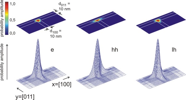
Figure 2.4.168 Probability amplitudes of the electron (e), heavy hole (hh) and light hole (lh) envelope functions at an unstrained T-shaped intersection of two 10 nm wide $\mathrm{GaAs}$ quantum wells embedded by ${\mathrm{Al}}_{0.35}{\mathrm{Ga}}_0.65\mathrm{As}$ barriers. The wave functions are normalized so that the maxima are equal to one.

Figure 2.4.169 Contour diagram of the probability amplitudes of the electron (e), heavy hole (hh) and light hole (lh) eigenfunctions (same figures as Figure 2.4.168, but this time viewed from the top). The wave functions are normalized so that the maxima are equal to one.

These results are in very good qualitative agreement with the heavy hole and light hole wave functions calculated within the 6-band k.p calculation This demonstrates the impact of an isotropic (for electrons and light holes) or anisotropic (for heavy hole) effective mass on the obtained wavefunctions.

Acknowledgement:

We would like to thank Robert Schuster from the University of Regensburg for providing experimental data and some figures for this tutorial.

---

Last update: 13/09/2024